
Exploration schemes in Deep Q-Networks (DQN)
Reimplementing well-known and successful Deep Reinforcement Learning (DRL) is probably well recommended, if not necessary step for any research in that field. One of the simplest DRL algorithm would be the Deep Q-Network developed at DeepMind. This algorithm was one of the first to demonstrate some learning on the domains of the Atari 2600 system provided by the Arcade Learning Environment.
While reimplementing this algorithm, a quite troublesome point I came across was the exploration mechanism used. Indeed, depending on the environment, some exploration schemes would work better than others.
In the following section, we present a handful of exploration schemes that can be combined with DQN and investigate their respective impact on the learning of the agent, as well as the speed of its convergence.
Impact of the exploration scheme on the DQN
Exploration schemes
First, we present the 4 exploration schemes investigated in this little side experiment.
1. Greedy exploration:
Following this exploration scheme, the agent will always take the action it considers best. This method is known to be vulnerable to the stuck local optimum problem, especially on the environment that requires “finesse” in exploration.
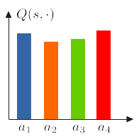
2. Botzmann-based exploration:
This method consists in using Categorical distribution (in this case, the one provided by the Pytorch framework) parameterized by the output of the Multilayer Perceptron that represents the agent’s policy.
To the best of my knowledge, the Categorical distribution already incorporates some randomness through the use of the sample() function we use to sample the actions during the training.
This enables the agent to sample sub-optimal action sometimes. While this technique is not “greedy”, it is still quite close to it since the parameterized network quickly becomes biased toward the action it evaluated as “best” in the early phase of the training, which is not always optimal, especially in harder tasks where it is hard to discover the optimal action in the first place.
The appeal of this method is namely the ease of its implementation (matches this one’s laziness).
3. $\epsilon$-greedy exploration
This exploration scheme consists in sampling with random action once in a while, instead of always using the greedy (and likely biased) sampling method described at 1. More specifically, we define a relatively small value $\epsilon < 1.0$, then, before sampling an action, randomly sampled from the uniform distribution on the interval $[0,1]$. If the randomly sampled value happens to fall below the predefined $\epsilon$, we take a random action, instead of taking the action that would maximize the expected discounted reward (according to the agent’s policy, i.e. the Q-Network). This ensures the agent keeps wandering in parts of the state space it would not explore if it were to blindly follow its “greedy”, and helps the agent to escape the local optima (at least on simple enough task). Furthermore, we experimented with tow variants of the $\epsilon$-greedy exploration.
3-a. Fixed $\epsilon$
As the name indicates, the epsilon stays during the whole training process. This can result in wasteful sampling, especially as the training progresses. Namely, as the number of environment interaction increases, the agent is likely to have learned a satisfactory enough policy, and can thus rely on its sampling method for the rest of the training and focus on the relevant part of the state space. This allows for a better fine-tuning and higher final performance overall.
3-b. Linearly annealed $\epsilon$
To mitigate the wasteful sampling that is likely to occur when the $\epsilon$ is a constant, annealing the latter as training progress was proposed. As the number of environment interaction increases, the agent is made to rely more and more on the policy it learned, reducing the random actions.
Experiments and Results
We initially investigated the impact of each exploration scheme in 4 toy problems provided by the OpenAI Gym package. Regarding the setting of the experiments, the non-annealed $\epsilon$-greedy exploitation scheme was trained with $\epsilon = 0.15$. For the linearly annealed $\epsilon$-greedy scheme, however, the $\epsilon$-constant was set to decay from $0.4$ to $0.01$ over the first 80% of the total training steps, after which the agent defaults back to a purely greedy policy.
1. CartPole-v0

First, given the straightforward nature of this toy problem, greedy exploration schemes seem to work best.
This is further reinforced by the fact that the non-annealed $\epsilon$-greedy performs poorly, while the linearly annealed one’s performance slowly increases as the $\epsilon$ decays. In retrospect, decaying over 80% of the total training step might be overly cautious. Reducing the interval on which the $\epsilon$ is decayed should be more efficient.
2. MountainCar-v0

Slightly similar to the CartPole-v0 environment, the greedy policy achieves the best reward in the fastest.
Surprisingly, the Boltzmann-based exploration scheme, although supposedly greedy, has the worst performance in this environment.
The non-annealed $\epsilon$-greedy policy seems to get stuck in a local optimum, while the linearly annealed one slowly improves and converges to the optimal policy, taking almost 70% more sample than the purely greedy policy. Here again, having the $\epsilon$ decay faster would likely result in a faster convergence.
3. Acrobot-v1

Again, despite being mostly identical to the pure greedy exploration scheme, the Botzmann=based exploration achieves the lowest performance. The purely greedy policy still achieves the highest return, with the non-annealed $\epsilon$-greedy, then the linearly annealed $\epsilon$-greedy policy following closely behind, in that order.
Here again, the same trend that suggests purely greedy policy is the best for relatively straightforward environments. $\epsilon$-greedy policy pay a price in sample efficiency in those case.
4. LunarLander-v2

In this environment, the greedier the policy, the higher the final performance. This is supported by the fact that the non-annealed $\epsilon$-greedy policy and the greedy policy achieved the “best” convergence as well as final results. The purely greedy policy however, seems to be quite unstable, as can be observed from the various dips in the performance of its curve. The non-annealed $\epsilon$-greedy has a more stable learning curve than the latter. The Boltzmann-based achieves around 25% of the best possible performance, surprisingly. Finally, the linearly annealed $\epsilon$-greedy exhibits a high variance and achieves the lowest performance of them all.
Next are some experiments
5. PongNoFrameskip-v4

The full experiment results can be accessed in the following WANDB project.
Concluding Remarks
So far, greedy policy performs the best on toy problems such as CartPole-v0 or MountainCar-v0. As the complexity rises, however, $\epsilon$-greedy policy ultimately comes out first, albeit such a method seems to be sensitive to the hyperparameters such as the value of $\epsilon$ itself, as well as how long we continue to sporadically sample random actions.
2020-06-04 Update After more investigation regarding the Boltzmann-based exploration scheme, it turns out the Q-values of a given state output by the Q-network are usually so close together, that the resulting probability distribution over the action becomes equivalent to a random policy. Hence, the corresponding agent performs poorly over the few environments it was tested on.
Coming next … ?
- A cleaned up version of the source code.
- Experimenting with the Parameter Space Noise for Exploration technique, which happened to work quite well in some DDPG experiments.
- Further investigating the Boltzmann-based with a temperature-based sampling to relax the action distribution a little bit more.
Leave a comment