
Masked Autoencoder for Distribution Estimation (MADE) Implementation and Experiments
Introduction
Using the pretext of numerous encounters with models imported from the deep unsupervising learning field, namely variational autoencoders (World Models [1]), distribution estimators (Diversity Is All You Need [2]), or RealNVP[3] ( which appears in the paper: Latent Space Policy for Hierarchical Reinforcement Learning [4]), it became apparent that a better understanding of such models would be required for more interesting research progress. An additional motivation would be the need for reinforcement learning to be even more autonomous and make better use of its experience, which seemingly requires better representation learning or models, which again, could be said to relate closely with unsupervised learning.
Following the CS294-158-SP19 Deep Unsupervised Learning course of the University of Berkeley, I set off to reproduce the Masked Autoencoder for Distribution Estimation (MADE) [5]. While it was advertised as a simple enough algorithm, it might not be necessarily the case, especially for a freshman in the sub-field. Without further delay, let us dive into the content of the paper and the step-by-step process of reproducing the proposed method, as well as fitting it to our specific needs.
MADE: Core concept
In unsupervised reinforcement learning, the focus is to recover the distribution of the data we are provided, to use on downstream tasks such as new sample generation, compression, and so on. A simple example would be the autoencoder, which aims at learning a compressed representation $Z \in \mathbb{R}^K$ from a set of observed variables ${X}, X \in \mathbb{R^D}$. In this case, $Z$ serves as an approximation for the original unobserved variable that was used to generate said data $X$. Once we have approximated that latent variable, we can sample from the corresponding latent space to generate new, but related samples, or just use the decoder part to improve the performance in a classification task (?). The following figure provides a more intuitive example of that mechanism.

The core idea of MADE builds on top of that concept. It leverages potential relationships that exist among the elements of the input variable $X$ to build a prediction model for each element of said input variable.
Indeed, if we consider the red pixel in the flower picture of Figure 2, knowing about all the preceding (blue) pixels can help us estimate its value more effectively (See Figure 2 below).

This property is formally referred to as “autoregression” (dependence on itself), and is implemented in MADE by introducing masks for the weights of the neural network that is used to estimate the distribution of the variable’s element. More concretely, this is achieved by masking all the pixels from the red one onward (grey pixels in the corresponding figure). The distribution of an arbitrary pixel thus becomes dependent on a few other pixels. While Figure 2 and the accompanying explanation consider the natural order of the pixel (namely we start from the upper-left corner, to the bottom-right one), MADE loosen this restriction to allow conditioning over and arbitrary order of pixel (or input variables). Intuitively, this can come in handy because we do not actually know what is the real auto-regressive relationship between the input variables. The natural order might not be the best, and to take Figure 2 as an example, predicting the value of the red pixel could be more effective if we conditioned on some of the pixels that come later (the grey ones).
In any case, we shall explore how it is achieved in the following section, as well as in the implementation section.
Technical details
Standard Autoencoder
Before actually diving into the method proposed in the paper, let us first quickly review the inner workings of an autoencoder, basing ourselves on a really simplified one illustrated in Figure 3.

For simplicity, we thus define the input $X$ of the neural network as a vector of 3 real variables such as: $X = \left( \matrix{x_1 & x_2 & x_3} \right)$.
To compute the unique layer, or in this case the latent $H = \left( \matrix{h_1 & h_2 & h_3 & h_4} \right)$, we will define the “input-to-hidden” weight matrix $W$ and the “input bias” vector $B$ as follows:
\[H = g \left( X \times W + B \right)\]or even more explicitly:
\[W = \left( \matrix { w_{11} & w_{12} & w_{13} & w_{14} \\ w_{21} & w_{22} & w_{23} & w_{24} \\ w_{31} & w_{32} & w_{33} & w_{34} }\right) \mathrm{and} \enspace B = \left( \matrix{ b_1 & b_2 & b_3 & b_4} \right)\]$H$ is thus obtained as follows:
\[H = \left(\matrix{h_1 \\ h_2 \\ h_3 \\ h_4} \right) = g( \left( \matrix{ x_1 w_{11} + x_2 w_{21} + x_3 w_{31} + b_1 \\ x_1 w_{12} + x_2 w_{22} + x_3 w_{32} + b_2 \\ x_1 w_{13} + x_2 w_{23} + x_3 w_{33} + b_3 \\ x_1 w_{14} + x_2 w_{24} + x_3 w_{34} + b_4 } \right)) \mathrm{,} \enspace (1)\]where $g$ is an non-linear activation function. It is worth keeping in mind, however, that (a) in general the latent dimension is set to be smaller than the input, otherwise, the neural network can just learn to “copy” the inputs, which defeats the original purpose, and (b) that the column vector $H$ was transposed for better readability. We do this to make the explanation of MADE’s core idea more intuitive later on. (Note: $H$ in Equation (1) is actually not a column vector in this case, but the former representation looked more intuitive.)
Then, to map from the latent $H$ to the output vector, in this case, the reconstructed input $\hat{X} = \left( \matrix{ \hat{x}_1 & \hat{x}_2 & \hat{x}_3} \right)$, we also declare the “hidden-to-output” weight matrix $V$ and the corresponding bias bector $C$ as below:
\[V = \left( \matrix { v_{11} & v_{12} & v_{13} \\ v_{21} & v_{22} & v_{23} \\ v_{31} & v_{32} & v_{33} \\ v_{41} & v_{42} & v_{43} }\right) \mathrm{and} \enspace C = \left( \matrix{ c_1 & c_2 & c_3} \right)\]The output $\hat{X}$ is then explicitly computed as follows:
\[\hat{X} = \sigma \left( H \times V + C \right)\]which can be further broken down as:
\[\hat{X} = \left( \matrix{ \hat{x}_1 \\ \hat{x}_2 \\ \hat{x}_3 } \right) = \sigma ( \left( \matrix{ h_1 v_{11} + h_2 v_{21} + h_3 v_{31} + h_4 v_{41} + c_1 \\ h_1 v_{12} + h_2 v_{22} + h_3 v_{32} + h_4 v_{42} + c_2 \\ h_1 v_{13} + h_2 v_{23} + h_3 v_{33} + h_4 v_{43} + c_3} \right)), \enspace (2)\]where $\sigma$ represents the activation of the output layer. When dealing with binary variables, $\sigma$ is effectively understood as the sigmoid function, which squashed whatever raw output is computed between $0$ and $1$.
From Equations (1) and (2), we already start seeing how each element of the output $\hat{x}_1$, $\hat{x}_2$, and $\hat{x}_3$ is related to the inputs $x_1$, $x_2$ and $x_3$. Namely, we can express each of one them as a function of the inputs:
\[\hat{x}_1 = f_1(x_1,x_2,x_3) \\ \hat{x}_2 = f_2(x_1,x_2,x_3) \\ \hat{x}_3 = f_3(x_1,x_2,x_3)\]The goal of MADE is to change the inner workings of the autoencoder neural network so that every element of the output is only dependent on a subset of the original inputs:
\[\hat{x}_1 = f_1' \\ \hat{x}_2 = f_2'(x_1) \enspace (3) \\ \hat{x}_3 = f_3'(x_1,x_2)\]The relations above assume we are following a natural ordering of the input variables. Additionally, we observe that $\hat{x}_1$ is basically a constant, as it depends only … on the bias weights of the last layer of the network we shall be using.
For the sake of completeness, let us quickly review the loss function of the standard autoencoder when the input is formed of binary variables. The objective is to have $\hat{X}$ be as close as possible to the original input $X$, the loss function must materialize the difference between those two. Since the output \(\hat{X} = \sigma(H \times V + C)\) is actually the probability of each of its elements being $1$, the Binary Cross Entropy loss function is adequate for our objective.
An intuitive explanation of how it works would as follows: let’s assume the original input to be $X = \left( \matrix{ 1 & 0 & 1} \right)$, and two candidate outputs $\hat{X}_1 = \left( \matrix{ 0.9 & 0.15 & 0.95 } \right)$ and $\hat{X}_2 = \left( \matrix{ 0.5 & 0.95 & 0.25 } \right)$. Since each element $\hat{x}_i, i \in {1,2,3}$ of either $\hat{X}_1$ or $\hat{X}_2$ gives us the probability of the $i$-th element of being $1$, it follows that $\hat{X}_1$ describes the original input $X$ more accurately. This result can be formally measured by using the Binary Cross Entropy (BCE) loss function, which we define as follows:
\[\mathrm{BCELoss}(X,\hat{X}) = - \sum_{i=1}^{\vert X \vert} \left( x_i \times \mathrm{log}(\hat{x}_i) + \left( 1 - x_i \right) \times \mathrm{log}(1 - \hat{x}_i) \right)\]Our previous conjucture is thus objectively justified as follows:
\[\mathrm{BCELoss}(X, \hat{X}_1) = 0.67 \\ \mathrm{BCELoss}(X, \hat{X}_2) = 2.20\]By design, this BCE loss function decreases when the prediction accuracy increases. Therefore, we apply can apply any gradient descent method to minimize set loss to fit our model (neural network) and obtain the best weight values that achieve our objective.
Autoregressive Autoencoder
Recall that in the simplest case, MADE proposes to predict the value of an arbitrary element $p(x_i)$ of $X$ based on the preceding elements $x_{<i}$. If we consider the joint probability of all the elements of the vector $X$, this property is defined as below:
\[p(X) = \prod_{i=1}^{\vert X \vert}p(x_i \vert x_{<i}) \mathrm{.}\]This is achieved by masking the weights of the neural network. Still using the simple autoencoder network introduced above, we would have:
\[H = g \left( X \times \left( W \odot M^W \right)+ B \right)\]and
\[\hat{X} = \sigma \left( H \times \left( V \odot M^V \right) + C \right)\]To define masks $M^W$ and $M^V$, we first need to decide on (1) an ordering for the inputs and (2) the connectivity of the various weights ($H$) that compose out network to the components not only the inputs $X$, but also the output $\hat{X}$. Regarding the input ordering aspect, we assume the natural ordering, as the bottom layer in Figure 4. For the hidden units, however, the original work proposes sampling from a uniform distribution between $1$ and $\vert X \vert - 1$. As per our example in Figure 4, we will use the ordering $\matrix{ 1 & 2 & 1 & 2}$ to further illustrate how the autoregressive property is achieved.
Once the orderings are decided, we can proceed to generate the weights, according to the following two rules:
(1) When computing the hidden units based on either the input vector $X$, or a previously hidden layer’s units: letting $k$ be the index of an arbitrary unit $h_k$, and $m(k)$ the connectivity number of said $k$-the element, we go over all the elements $d$ of the ordering (or connectivity number) of the previous layer. For simplicity, let is consider the ordering of the first component $x_1$, which is $d=1$. Further, we consider the first hidden unit $h_1$ (so $k$ = 1) of the hidden layer $H$. If $m(k)$ is greater or equal to an arbitrary $d=1$, this means that we allow the $k-th$ element of the hidden layer to dependent on that $x_1$. Since we are currently considering only $x_1$ and $h_1$, it follows that $m(1) > 1$. This corresponds to letting the weight $w_11$ as per Equation (1) (the $h1$ line) be as it is, which corresponds to a masking value of $1$. Therefore, any downstream operation that will use the value of $h_1$ will have a dependency on the $x_1# element.
Now, for the opposite case, consider the element $x_3$, with ordering $3$, while maintening $h_1$. Since $3$ is greater than any $m(1)$ of that hidden layer (recall that $m(k) \in {1,2}, \forall k$), we want to nullify the weight $w_31$, so that $h_1$ has no relation with $x_3$. Therefore, we attribute the value $0$ to the corresponding masking element of $M^W$. Such mask generation process is formally defined by the authors as follows:
\[M_{k,d}^{W} = 1_{m(k) \geq d} = \Bigg\{ \matrix { 1 \enspace \mathrm{if} \enspace m(k) \geq d \\ 0 \enspace \mathrm{otherwise} }\]Considering our simple autoencoder network in Figure 3, we would obtain the mask:
\[M^W = \left( \matrix { 1 & 1 & 1 & 1 \\ 0 & 1 & 0 & 1 \\ 0 & 0 & 0 & 1 }\right)\]and the hidden layer would thus be obtained by with the mask augmented computation $H = g \left( X \times \left( W \odot M^W \right)+ B \right)$, resulting in the hidden layer as speficied below:
\[H = \left(\matrix{h_1 \\ h_2 \\ h_3 \\ h_4} \right) = g( \left( \matrix{ x_1 w_{11} + b_1 \\ x_1 w_{12} + x_2 w_{22} + b_2 \\ x_1 w_{13} + b_3 \\ x_1 w_{14} + x_2 w_{24} + b_4 } \right)) = \left(\matrix{f^h_1(x_1) \\ f^h_2(x_1,x_2) \\ f^h_3(x_1) \\ f^h_4(x_1, x_2)} \right) \mathrm{.}\]The last column explicitly shows the dependence of each component $h_i$ on the inputs. So far so good.
(2) Recall that when computing the outputs $\hat{X}$ based on the last hidden layer ($H$ in this case), we want to make sure that element $\hat{x}_2$ only depends on $x_1$, or more explicitly as per Equation (3). To do so, the authors propose to first attribute the input ordering to the output too. Then the following formula is used do generate the mask that will realize the autoregressive property in the output.
\[M_{d,k}^{V} = 1_{d > m(k)} = \Bigg\{ \matrix { 1 \enspace \mathrm{if} d > m(k) \\ 0 \enspace \mathrm{otherwise} }\]Intuitevely, let us consider the hidden layer’s component $h_2 = f^h_2(x_1,x_2)$, and try to find which output component $\hat{x}_i$ should be connected to it. Since $x_1$ is supposed to represent the estimate of $p(x_1)$, it must not depend on any of the $x_i$. Therefore, the weight that connects $h_2$ to $\hat{x}_1$ must be set to $0$. $x_2$, however, estimates $p(x_2\vert x_1)$, therefore it cannot depend on $h_2$, since the latter depends on $x_2$. The corresponding weight must thus be set to $0$ again, and the same goes for $h_4$ in fact. Since $h_1$ and $h_3$ only depend on $x_1$, the weights connecting those two to $x_2$ can bet set to $1$.
Again, for our simple autoencoder’s output weights $V$, we would obtain the mask:
\[M^V = \left( \matrix { 0 & 1 & 1 \\ 0 & 0 & 1 \\ 0 & 1 & 1 \\ 0 & 0 & 1 }\right)\]and the computation $\hat{X} = \sigma \left( H \times \left( V \odot M^V \right) + C \right)$ can be decomposed as follows:
\[\hat{X} = \left(\matrix{ \hat{x}_1 \\ \hat{x}_2 \\ \hat{x}_3 } \right) = \sigma( \left( \matrix{ c_1 \\ h_1 v_{12} + h_3 v_{32} + c_2 \\ h_1 v_{13} + h_2 v_{23} + h_3 v_{33} + h_4 v_{43} + c_3 } \right)) = \left( \matrix{f^v_1 \\ f^v_2(x_1) \\ f^v_3(x_1,x_2)} \right) \mathrm{,}\]which is exactly the result that is aimed for in Equation (3). Pictorially, this is illustrated as the following figure.

Also notice how the $x_3$ element is never used for prediction, as it should be. Furthermore, despite $\hat{x}_1$ being independent of any input $x_i$, it can still model a distribution by relying on the bias weights $C$ of the output layer. Also, while the masking makes the connectivity in the network sparser (especially when compared with Figure 3), the resulting neural network is usually still powerful enough the model the distributions of the output. Worse case, we can always add more layers to make up for that sparsity.
Finally, it is important to note that while the example above relies on the natural ordering of the input, in practice, we might benefit by using a different, random ordering for example. This is also taken into account by the authors in the papers, where the also propose to permute the ordering of the inputs, and use it to generate the masks.
Similarly, only using a single set of connectivity count for the components of the hidden layers, a different parameterization might give us better results by capturing the autoregressive property more accurately. To address this problem, MADE is trained in a connection agnostic fashion, namely by intermittently generating new connectivity count for the hidden layers during the training. The final model is then evaluated across all those different orderings. Such a method contribute to a more robust model, as the latter has to fit its weights so as to support different configurations of its hidden layers.
We shall now introduce a simple implementation for the masked autoencoder in the next section.
Implementation, Experiments and Results
We first apply the MADE technique to reconstruct digits from the MNIST dataset, as per the original work, using the Python programming language and the Pytorch Deep Learning framework. (Full code and results)
1. Binarized MNIST Digits modeling using MADE
Let us first define a few dependencies as follows:
# Dependencies
import random
import numpy as np

# Pytorch support
import torch as th
import torch.nn as nn
import torch.optim as optim
import torch.nn.functional as F

from torchvision import transforms, datasets
from torchvision.utils import make_grid

import matplotlib.pyplot as plt
This makes available the various libraries that will be used to generate or read the data, create the neural networks, and train them, as well as plot the results.
Next, we declare a few hyperparameters that will among which the architecture of the neural networks, the orderings of the input, the number of masks to use for the layer masking.
# Hyper parameters
SEED = 42
N_EPOCHS = 200
LR = 1e-3
BATCH_SIZE = 128

HIDDEN_SIZES = [512,512]
LATENT_DIM = HIDDEN_SIZES[-1]

INPUT_ORDERINGS = 0
 # Input ordering meaning
# -1: Generate a new input ordering every time it is needed. Not realistic.
#  0: Natural Order
#  1: A single input ordering but shuffled
#  2..:  Does that even make sense to sample multiple ordering throughout training? Only feels like it is gonna confuse the network on what input is what ...

CONNECTIVITY_ORDERINGS = 1
# connectivity Orderings
# -1: Generate new masks everytime. Unrealistic
#  0: Equivalent to vanilla autoencoder
#  1..: Use specified amount of randomly generated masks.

RESAMPLE_INTERVAL = 20

USE_GPU=True
device = th.device( "cuda" if th.cuda.is_available()and USE_GPU else "cpu")

# Seeding
random.seed(SEED)
np.random.seed( SEED)

# Pytorch seeding
th.manual_seed( SEED)
if device.type == "cuda":
    th.cuda.manual_seed_all(SEED)
We can now format the data to facilitate the training loop, now that we have defined the BATCH_SIZE hyperparameter.
# Data loading
mnist = np.load("binarized_mnist.npz")
train, test = mnist['train_data'], mnist['valid_data']

train = th.from_numpy(train).to(device)
test = th.from_numpy(test).to(device)

trainset = th.utils.data.DataLoader( train, batch_size=BATCH_SIZE, shuffle=True)
testset = th.utils.data.DataLoader( test, batch_size=BATCH_SIZE, shuffle=False)
Entering the most challenging part, we create the MADE model, by implementing the input ordering as well as the mask generation, as well as the mask application method.
# Model
INPUT_DIM = 28**2
OUTPUT_DIM = 28**2

# Augmenting the nn.Linear to support masks
class MaskedLinear(nn.Linear):
    def __init__(self, in_features, out_features, bias=True):
        super().__init__(in_features, out_features, bias)
        self.register_buffer('mask', th.ones(out_features, in_features))

    def set_mask(self, mask):
        self.mask.data.copy_(th.from_numpy(mask.astype(np.uint8).T))

    def forward(self, input):
        return F.linear(input, self.mask * self.weight, self.bias)

class EncoderDecoder(nn.Module):
    def __init__(self):
        super().__init__()

        # Dynamic generating of mask and orderings for efficiency
        self.connectivity_ordering_seed = 0
        self.input_ordering_seed = 0

        # Pay attention to the "s"
        self.connectivity_orderings = CONNECTIVITY_ORDERINGS
        self.input_orderings = INPUT_ORDERINGS

        # MLP Layers
        self.encoder_layers = nn.ModuleList()
        self.decoder_layers = nn.ModuleList()

        # Hidden sizes presistent
        self.encoder_hiddens = HIDDEN_SIZES
        self.decoder_hiddens = HIDDEN_SIZES[::-1][1:]
        self.decoder_hiddens.append(INPUT_DIM)

        # This define d for each component of the input vector
        self.input_ordering = [ i for i in range(1,INPUT_DIM+1)] # m_0 in the paper

        current_dim = INPUT_DIM
        current_input_orders = self.input_ordering # (m_l in the paper)

        ## Encoder layers
        for hsize in self.encoder_hiddens:
            # Linear layer with weights and biases included
            self.encoder_layers.append( MaskedLinear(current_dim, hsize))

            current_dim = hsize

        ## Decoder layers
        for hsize in self.decoder_hiddens:
            # Linear layer with weights and biases included
            self.decoder_layers.append( MaskedLinear(current_dim, hsize))

            current_dim = hsize

        ## Input ordering: if only using one random shuffling, do it here,
        # then skip it in the shuffling function for efficiency
        if self.input_orderings == 1:
            np.random.shuffle(self.input_ordering)

        # Let's us know if the mask was generated at least once already, for efficiency when using a single connectivity ordering
        self.mask_generated = False

        self.generate_masks()

    # This is left for reference. Not actually used.
    # The idea is to also shuffle the input ordering as training goes along, but intuitively, it seems too unstable
    def shuffle_input_ordering(self):
        # Totally random input ordeing generation. Quite unstable
        if self.input_orderings == -1:
            random.shuffle(self.input_ordering)

        if self.input_orderings in [0,1]:
            pass # Using natural order

        elif self.input_orderings > 1:
            rng = np.random.RandomState(self.input_ordering_seed)

            self.input_ordering = rng.randint(1, input_dim+1, input_dim)
            self.input_ordering_seed = (self.input_ordering_seed + 1) % self.input_orderings
        else:
            raise NotImplementedError

    def generate_masks(self):
        if self.mask_generated and self.connectivity_orderings == 1:
            return # Skips mask generation for efficiciency

        if self.connectivity_orderings == -1:
            raise NotImplementedError

        elif self.connectivity_orderings >=1:
            # Inspired from Andrej Karpathy's implementation. Props where due.
            rng = np.random.RandomState(self.connectivity_ordering_seed)
            self.connectivity_ordering_seed = (self.connectivity_ordering_seed + 1) % self.connectivity_orderings

        else:
            raise NotImplementedError

        current_dim = INPUT_DIM
        current_input_orders = self.input_ordering # (m_l in the paper)

        layer_connect_counts = []

        for layer_idx, hsize in enumerate(self.encoder_hiddens):
            # Fix #1: Make sure we do not sample connectivity count that are not in the previous layer,
            # since they won't be useful, and reduce the number of weights that are actually used for the esitmation
            layer_count_low = 1 if len(layer_connect_counts) == 0 else np.min(layer_connect_counts)
            layer_connect_counts = [rng.randint(low=layer_count_low,high=INPUT_DIM) for _ in range(hsize)]

            # Generating a mask for each layer and storing it
            mask = [[ 1 if layer_connect_counts[k] >= d else 0 for k in range(hsize)] for d in current_input_orders]
            self.encoder_layers[layer_idx].set_mask(np.array(mask))

            current_dim = hsize
            current_input_orders = layer_connect_counts

        # Decoder subsection
        for layer_idx, hsize in enumerate(self.decoder_hiddens):
            if layer_idx == len(self.decoder_hiddens)-1:
                layer_connect_counts = self.input_ordering
                mask = [[ 1 if layer_connect_counts[k] > d else 0 for k in range(hsize)] for d in current_input_orders]
            else:
                # Note: In case we did not reach the last layer, we still generate the mask as for the
                # encoder's layer ! That was the problem we were having ...
                layer_count_low = 1 if len(layer_connect_counts) == 0 else np.min(layer_connect_counts)
                layer_connect_counts = [rng.randint(low=layer_count_low,high=INPUT_DIM) for _ in range(hsize)]

                # Generating a mask for each layer and storing it
                mask = [[ 1 if layer_connect_counts[k] >= d else 0 for k in range(hsize)] for d in current_input_orders]

            self.decoder_layers[layer_idx].set_mask(np.array(mask))

            current_dim = hsize
            current_input_orders = layer_connect_counts

        self.mask_generated = True

    def encode(self,x):
        for layer in self.encoder_layers:
            x = F.relu(layer(x))

        return x

    def decode(self,z):
        for layer in self.decoder_layers[:-1]:
            z = F.relu(layer(z))

        z = self.decoder_layers[-1](z)

        return th.sigmoid(z)

    def forward(self,x):
        # Full pass
        return self.decode(self.encode(x))

encdec = EncoderDecoder().to(device)

print( encdec)

optimizer = optim.Adam(list(encdec.parameters()), lr=LR)
With the default hyperparameters, we get the following MADE model:
EncoderDecoder(
  (encoder_layers): ModuleList(
    (0): MaskedLinear(in_features=784, out_features=512, bias=True)
    (1): MaskedLinear(in_features=512, out_features=512, bias=True)
  )
  (decoder_layers): ModuleList(
    (0): MaskedLinear(in_features=512, out_features=512, bias=True)
    (1): MaskedLinear(in_features=512, out_features=784, bias=True)
  )
)
We can now proceed to the training loop of the model:
# Helper to compute loss function
def compute_loss(model, data):
    x_pred = model(data)

    loss = F.binary_cross_entropy(x_pred, data)

    return loss

def compute_test_loss(model, testset):
    loss = 0.
    for test_batch_idx, test_batch in enumerate(testset):
        loss += compute_loss(model, test_batch.to(device))

    loss /= (test_batch_idx+1)

    return loss

# Training loop

# Holders for logging statistics. Maybe disregarded at first
batch_iter = 0 # Used as a reference to regenerate masks
mb_train_losses = []
test_losses = []

test_loss = compute_test_loss( encdec, testset)
test_losses.append( test_loss.item())

# Note. Used to correct the sampling order especially when the input ordering is not natural
IDX_TO_ORDERING = {}
for idx in range(INPUT_DIM):
    for comp_idx, comp in enumerate(encdec.input_ordering):
        if comp == idx+1:
            IDX_TO_ORDERING[idx] = comp_idx
            break # for efficiency

for epoch in range( N_EPOCHS):

    # Iterate over minibatches
    for mb_idx, mb_train_data in enumerate(trainset):

        # Train the MADE model
        mb_train_loss = compute_loss(encdec, mb_train_data.to(device))

        optimizer.zero_grad()
        mb_train_loss.backward()
        optimizer.step()

        mb_train_losses.append(mb_train_loss.item())

        batch_iter += 1
        if batch_iter % RESAMPLE_INTERVAL == 0:
            encdec.generate_masks()

    # Logging stats: Compute the test / validation loss over the full test batch only at the epoch's end.
    test_loss = compute_test_loss( encdec, testset)
    test_losses.append( test_loss.item())

    print( "Epoch %d (Last MB Loss)" % (epoch))
    print( "\t Train Loss : %.4f , Test Loss: %.4f" %( mb_train_loss, test_loss))

    # Plotting.
    if (epoch > 0 and epoch % 1 == 0) or epoch == (N_EPOCHS -1):
        fig, axes = plt.subplots(1, 2,figsize=(16,8))

        x_mbs_train = np.arange(len(mb_train_losses))
        x_mbs_test = np.arange(0, len(mb_train_losses), mb_idx) # Test loss at the end of each epoch needs to account for gap in minibatch

        # Ploting train and test losses
        axes[0].plot(x_mbs_train, mb_train_losses,label="MADE Train MB Loss")
        axes[0].plot(x_mbs_test, test_losses,label="MADE Test Loss")
        axes[0].set_xlabel("Minibatches")
        axes[0].set_ylabel("BCE Loss")
        axes[0].set_title("Train and Test losses")
        axes[0].legend()
        axes[0].grid(True)

        # Sampling from the MADE model
        ## Plot parameterization
        N_EVAL_SAMPLES = 100
        N_ROW = int(math.sqrt(N_EVAL_SAMPLES))
        N_ROW += N_EVAL_SAMPLES % N_ROW # In case there are some left over, add an additional row

        with th.no_grad():
            final_sample = th.rand([N_EVAL_SAMPLES, INPUT_DIM]).to(device)
            # Note that we sample in Parallel ! which is much faster. That is why we use the [:, corrected_idx]
            # This restricts it to the using a single mask, however.

            for sampled_idx in range(INPUT_DIM):
                corrected_idx = IDX_TO_ORDERING[sampled_idx]
                reconstructed = encdec(final_sample)
                reconstructed = th.bernoulli(reconstructed) # Properly discretized the output to get concrete results
                final_sample[:, corrected_idx] = reconstructed[:, corrected_idx]

            # Some reshaping and prettifying
            final_sample = final_sample.view([N_EVAL_SAMPLES,1,28,28])
            final_sample = make_grid(final_sample, nrow=N_ROW).cpu().numpy()
            final_sample = np.moveaxis(final_sample, (0,1,2), (1,2,0))
            final_sample = np.moveaxis(final_sample, (0,1,2), (1,2,0))

            axes[1].imshow(final_sample)
            fig.tight_layout()
            plt.show()
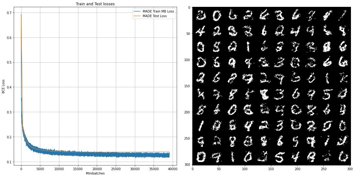
The results of training documented below, with a training loss that converges to around 88.0 (negative log-likelihood), and sampled digits similar to the original work.
The full source code, as well as the results, can be founded and interacted within the following Collab Notebook.
Some implementation notes
- When computing the test loss at first, it was done using the whole $10000$ samples at once. While the results were correct, it created a (GPU) memory leak that disallowed training for too many epochs, namely by causing an Out Of Memory memory when using a GPU, and grind the system down to an irresponsive state when using the system memory combined with CPU computation (No GPU). The choice was thus made to also evaluate using small batch at a time for the testing too.
- Sampling from the MADE model follows a really special procedure: since each element of the output is constrained between $0$ and $1$, as it is a probability, just plotting the resulting vector as one would do when using a standard VAE would result the same blurry picture.
reconstructed = encdec(final_sample)
reconstructed = th.bernoulli(reconstructed) # Properly discretized the output to get concrete results
To obtain an actual picture of a digit, the output of the model has to be fed to a Bernoulli distribution, from which we draw samples, as per the following code extracted from above. This is probably why the dataset is characterized as binarized MNIST: the actual values of each pixel, be it in the data or in the correctly sampled output are either 0 or 1, disallowing any shade of grey.
- When using a * non-natural ordering* for the inputs, the sampling process has to be adapted according to so that the correct element is sampled as we iterate over each component of the output vector. In this case, this was achieved by building a mapping from component index to the ordering as per:
IDX_TO_ORDERING = {}
for idx in range(INPUT_DIM):
    for comp_idx, comp in enumerate(encdec.input_ordering):
        if comp == idx+1:
            IDX_TO_ORDERING[idx] = comp_idx
            break # for efficiency
then using that map to access the data at the index we are currently sampling as in the following section of code extracted from above.
for sampled_idx in range(INPUT_DIM):
    corrected_idx = IDX_TO_ORDERING[sampled_idx]
    reconstructed = encdec(final_sample)
    reconstructed = th.bernoulli(reconstructed) # Properly discretized the output to get concrete results
    final_sample[:, corrected_idx] = reconstructed[:, corrected_idx]
2. Two Dimensional data modeling with MADE using categorical distribution
Next, we apply the MADE model to some data given in Exercise 2 of the Spring 2019 Deep Unsupervised Learning Week 1 Homework course of the University of Berkeley. The goal is to use the autoregressive property to model the distribution of the provided data, which is represented as a two-dimensional vector. Each component of the vector, however, takes a discrete value between $0$ and $199$. Therefore, we adapt the MADE to model a categorical distribution for each component of said vector, while retaining the autoregressive property.
Furthermore, we also experiment with various format of the input, namely (a) left as is, (b) normalized input, and finally (c) one-hot vectors for each $x_1$ and $x_2$. Using (c) as the representative case, we review the parts of the model presented in the previous MNIST case. The source code for the latter case is available as the following Google Colab Notebook.
First, the declaration of the model input-to-hidden and hidden-to-output layers have to be revised according to the new output dimension, and take into account the fact that the output for each component $x_i$ becomes their respective probability distributions over the range of values $0$ to $199$. An especially important part is how to make sure the mask input ordering is correctly extended to match the one-hot vector input. Fortunately, once it is done, it also takes care of the ordering of the extended output vector that is used to model the respective distribution of the $\hat{x}_i$ components.
As a practival example, letting $X = \left( \matrix {x_1 & x_2} \right) = \left( \matrix{144 & 12} \right)$, and the correspponding natural input ordering $\left( \matrix{1 & 2} \right)$. Extended to a one hot vector: $X^{hot} = \left( [ \matrix {0 & 0 & 0 & \mathrm{…} & 1 & \mathrm{…} & 0} ] , [\matrix{0 & 0 & 0 & 0 & 0 & 0 & 0 & 0 & 0 & 0 & 0 & 1 & \mathrm{…} & 0}] \right)$. Concatenating this gives us a vector of dimension $200 \times 2 = 400$, and the corresponding input ordering would thus be: $\left( \matrix{ 1 & 1 & 1 & \mathrm{…} & 1 & 2 & 2 & 2 & \mathrm{…} & 2}\right)$ (the first 200 are elements are 1, while the remaining 200 are 2). Pictorially, we get the model represented in the figure below:

The implementation introduced above for the MNIST example is modified to fit this problem. The updated part is presented in the simplified code section below.
# Model definition
INPUT_DIM = 2
N_CLASSES = 200 # Used to tranform the inputs into one-hot vectors
OUTPUT_DIM = INPUT_DIM * N_CLASSES # We aim at having the prob dist for each x1 and x2 component...

class MaskedLinear(nn.Linear):
    # ... same as MNIST ...

class EncoderDecoder(nn.Module):
    def __init__(self):
        super().__init__()
        # ... same as MNIST ...

        # This define d for each component of the input vector
        # Since we are using the one hot input format, we need to adjust the layer connectivity ordering
        self.input_ordering = []
        for i in range(1,INPUT_DIM+1):
            for _ in range(N_CLASSES):
                self.input_ordering.append(i)

        current_dim = INPUT_DIM * N_CLASSES
        current_input_orders = self.input_ordering # (m_l in the paper)

        # ... same as MNIST ...

        self.generate_masks()

    def shuffle_input_ordering(self):
        # ... same as MNIST ...

    def generate_masks(self):
        # ... same as MNIST ...

        # Account for the dimensional change of the input due to the one-hot input.
        # The rest follows naturally when generating the masks

        current_dim = INPUT_DIM * N_CLASSES
        current_input_orders = self.input_ordering # (m_l in the paper)

        # ... same as MNIST ...

    def encode(self,x):
        # ... same as MNIST ...

    def decode(self,z):
        for layer in self.decoder_layers[:-1]:
            z = F.relu(layer(z))

        z = self.decoder_layers[-1](z)

        # Separate the logits of the distribution for x_1 and x_2, so as to construct their respective probability distribution
        # The masking is already taking care of by generating the "self.input_ordering" as in the __init__() method above.

        x1_logits = z[:, :N_CLASSES]
        x2_logits = z[:, N_CLASSES:]

        return x1_logits, x2_logits

    def forward(self,x):
        # ... same as MNIST ...

# Instanciating the model
encdec = EncoderDecoder().to(device)
print(encdec) # DEBUG

# Optimizer
optimiza = optim.Adam(list(encdec.parameters()), lr=LR)
Since we are now dealing with multiple classes, we also need to adjust the loss computation to the cross-entropy instead. We must also make sure to properly separate the respective distributions of $x_1$ and $x_2$, as well as their label data when computing said loss. Pragmatically, this is achieved as demonstrated in the code section below.
# Helper to compute loss function
def compute_loss(model, data):
    x1s = data[:,0]
    x2s = data[:,1]

    # One hot and concatenante
    x1s_hot = F.one_hot(x1s, N_CLASSES).float()
    x2s_hot = F.one_hot(x2s, N_CLASSES).float()
    data = th.cat([x1s_hot,x2s_hot], 1)

    z = model.encode(data)

    x1_logits, x2_logits = model.decode(z)

    x1_loss = F.cross_entropy(x1_logits, x1s)
    x2_loss = F.cross_entropy(x2_logits, x2s)
    loss = x1_loss + x2_loss

    return loss, z.detach()
Finally, we can proceed to the actual training of the network. While the optimization phase is basically the same as the MNIST case once we have adapted the model structure and the loss, the sampling from the MADE model has to also be changed to take into account the categorical distributions of the input variables $x_1$ and $x_2$.
# Training loop
mb_train_losses = []
test_losses = []
test_loss, _ = compute_loss( encdec, test_batch)
test_losses.append( test_loss.item())
# for epoch in range( n_epochs):
for epoch in range( N_EPOCHS):
# ... same as MNIST ...
print( "Epoch %d (Last MB Loss)" % (epoch))
print( "\t Train Loss : %.4f , Test Loss: %.4f" %( mb_train_loss, test_loss))
if (epoch > 0 and epoch % 1 == 0) or epoch == (N_EPOCHS -1):
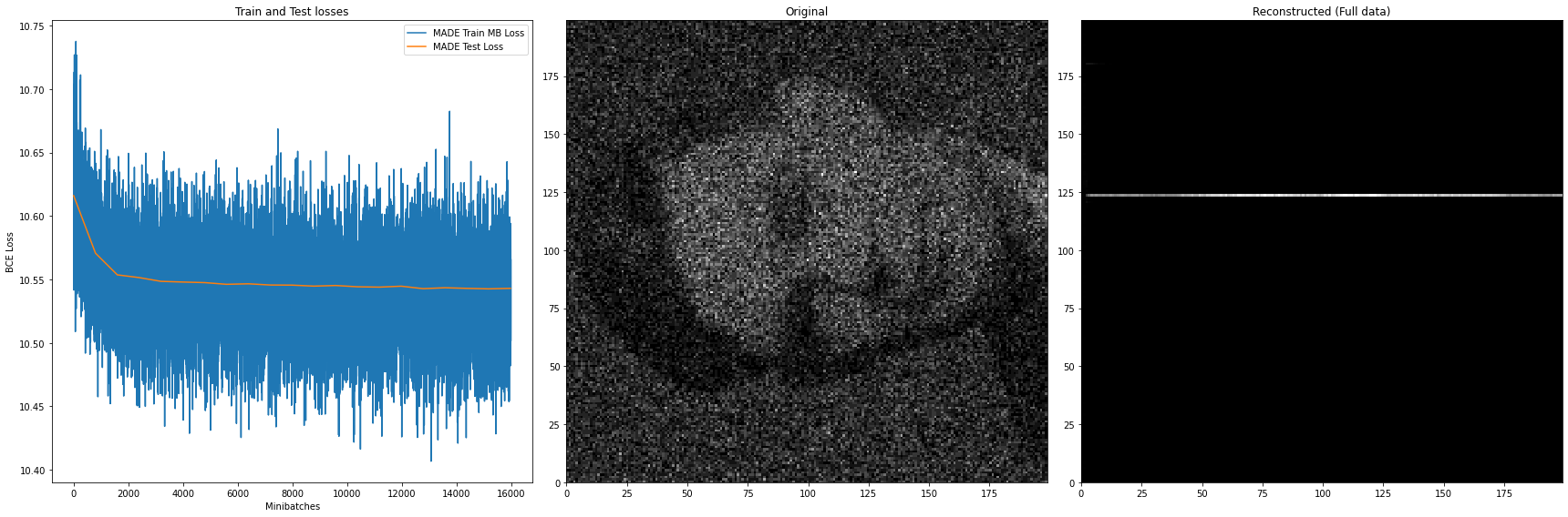
fig, axes = plt.subplots(1, 3,figsize=(24,8))
x_mbs_train = np.arange(len(mb_train_losses))
x_mbs_test = np.arange(0, len(mb_train_losses), mb_idx) # Test loss at the end of each epoch needs to account for gap in minibatch
# Ploting train and test losses
axes[0].plot(x_mbs_train, mb_train_losses,label="MADE Train MB Loss")
axes[0].plot(x_mbs_test, test_losses,label="MADE Test Loss")
axes[0].set_xlabel("Minibatches")
axes[0].set_ylabel("BCE Loss")
axes[0].set_title("Train and Test losses")
axes[0].legend()
# Plotting sampled points and original on the left
axes[1].hist2d( full_data[:,0], full_data[:,1], bins=(200,200), cmap='gist_gray')
axes[1].set_title('Original')
# Sampling from the MADE and reconstructing the data
with th.no_grad():
## Get P_\theta(x_1) and sample from it
dummy_input = th.zeros([1, INPUT_DIM * N_CLASSES]).to(device)
x1s_pred, _ = encdec(dummy_input)
x1_estimate_samples = Categorical(logits=x1s_pred).sample([len(full_data)]).squeeze()
x1_estimate_samples_hot = F.one_hot(x1_estimate_samples, N_CLASSES).float()
x1_estimate_samples_hot = th.cat([x1_estimate_samples_hot,
th.zeros([x1_estimate_samples_hot.shape[0], N_CLASSES]).to(device)], 1) # Adds the expected x2 one hot
# Get P(x_2|x_1) and sample the corresponding x2 to comple the pairs
_, x2s_pred = encdec(x1_estimate_samples_hot)
x2_dist = Categorical(logits=x2s_pred)
x2_estimate_samples = x2_dist.sample() # Dimension deduced from x1s estiamted sample shape ! So nice of pytorch
# Type fix
x1_estimate_samples = x1_estimate_samples.cpu().numpy()
x2_estimate_samples = x2_estimate_samples.cpu().numpy()
axes[2].hist2d( x1_estimate_samples, x2_estimate_samples, bins=(200,200), cmap='gist_gray')
axes[2].set_title('Reconstructed (Full data)')
axes[2].set_xlim(0, 199)
axes[2].set_ylim(0, 199)
fig.tight_layout()
plt.show()
# Shuffle the data in a K-folding style, but without the K.
if SHUFFLE_DATA:
trainset, test_batch = shuffle_dataset()
After training for just 20 epochs, the model can already reconstruct (right plot) the original data (middle plot) quite well enough. The loss however, while still quite high in variance, exhibits a slight decrease.
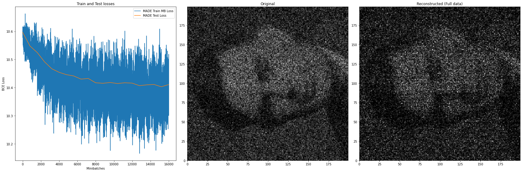
Using MADE definitely gets us better results than when using a naive non-autoregressive model of the form $\tilde{p}(x_1, x_2) = \tilde{p}(x_1)\tilde{p}(x_2 \vert x_1)$, as illustrated in the Figure 8 below.
Some additional remarks
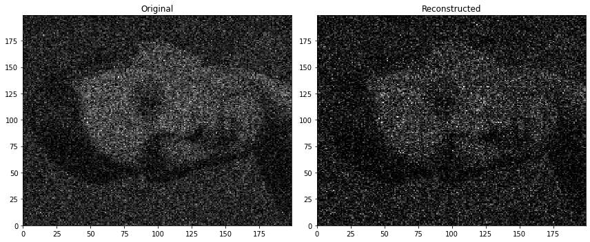
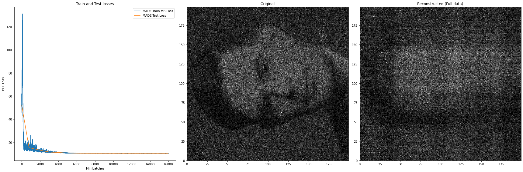
- The case (c) where the input are encoded as a one-hot vector was selected as the representative case because the other cases, namely (a) input left as is (values of $x_1$ and $x_2$ ranging froom $0$ to $199$), and (b) normalized input, performed comparatively worse. Interestingly, the normalized input version (Figure 10) struggled to reconstruct the provided dataset even more than the one without normalization (Figure 9).
For the sake of completeness, the complete source code files are provided in the form of a Google Colab Notebook for playing around with the various parameterization.
Discussion and Conclusion
This concludes our dive into the MADE’s inner workings, as well as experiments conducted on the MNIST digits dataset with continuous outputs, and a custom dataset with two-dimensional input data with discrete outputs. In both case, MADE can be used to generate new samples while leveraging the autoregressive property between elements of the input.
Some additional remarks
- Realizing the autoregressive property using the masking method proposed in method is likely making some weights useless, since they always end up being multiply by $0$ and not contributing to the gradient. For small enough inputs, standard size neural networks( 2 layes of 512 units for example) seems to work well enough thanks to the universal approximation property of neural networks. For higher dimensional inputs, increasing the depth of the network, as well as the width of the layers should also increase the number of weights actually used for the computations, thereby increasing the expressiveness of the models.
- Following the MNIST experiment, it is important to notice that when the width of the layers are lesser than the dimension of the input vector, some input are likely to not be used during the autoregression, therby losing some potentially important relationships that exist in the input. Similarly, it is not clear if sampling the connectivity counts of the hidden layers using a uniform distribution actually gives us a good autoregression with respect to the given dataset. For example, the output image might be highly dependent on the say the range $[200,400]$ in the case of the MNIST digit dataset (somewhere around the center of the picture). Therefore, having more values sampled from that range could create a more usefull autoregression and lead to better results when generating new samples. This could be achieved by using a different distribution to generate the connectivity counts for those hidden layers, or applying some constraint based on some prior knowledge. This would however be quite time and resource consuming, thus using the uniform distriution is a general and “fair” method that works pretty well. Using it should not be that bad after all. (As they say: “If it ain’t broken, don’t fix it”).
- Personnaly, this took more time to undestand and implement than I would like to admit. The assignments were expected to be delivered in 1 or 2 weeks, but just this MADE exercise took me months, so that would have been a definite fail. Nevertheless, lesson learned.
The data for the models as well as the source code can be accessed in the following Google Drive folder, or GitHub repository.
Acknowledgments
- The original authors of the MADE paper for publish their works, as well as their source code, albeit a little bit cryptic for me.
- The enlightning explanation provided by the instructors of the CS294-158-SP19 Deep Unsupervised Learning course, especially how to sample from a MADE model with with categorical distributions as outputs.
- Sir Karpathy’s PyTorch implementation of MADE, which was tremendously useful as reference and for sanity checks.
- Google Collab for the (partial) computational resources.
Leave a comment