
Deep Deterministic Policy Gradient
Introduction
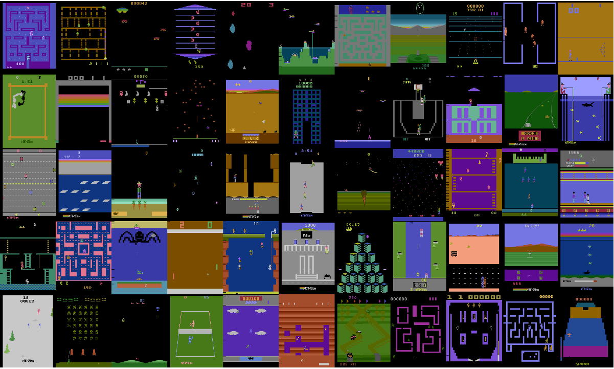
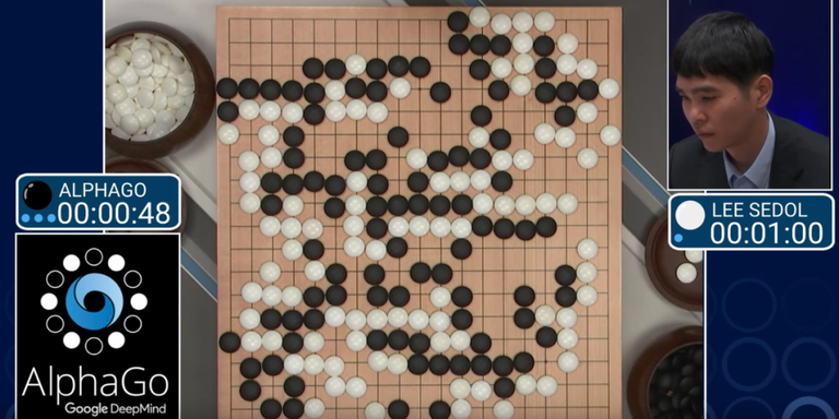
In the last few years, Deep Reinforcement Learning (DRL) has shown promising results when it comes to playing games directly from pixels ([1],[2]), mastering quite a few board games such as Chess, Go, and Shogi ([3]),as well as robotic control ([4], [5], [6]).
In the latter case, the control of the robot requires really precise control of actuators. Depending on the complexity of the robot’s frame, which can usually be reduced to its degree of freedom, the complexity of the actuation rises exponentially, and it becomes hard to design a control system with classical control theory. The appealing point of Deep Reinforcement Learning, in this case, is that it would allow us to learn such a control system, tailored to the desired task from scratch. This is expected to be achieved by having the agent interact with the environment of the given task, and find an “optimal way of doing things” (optimal policy in the Reinforcement Learning / Control Theory jargon) which achieves the given objective, simply via repetitive trial and errors, as an animal or a human would do.
Easier said than done, however, for techniques that can mostly be considered as classics now, such as policy gradients and (deep) Q-networks do not scale well to high-dimensional tasks, which we are interested in. At the cost of a slight repetition, the concern here is mainly the continuous nature of the action space, which makes learning a satisfactory enough policy difficult. Consequently, building on top of the Deep Q-Network ([1]), the Deep Deterministic Policy Gradients introduces a method which at least exhibits some learning in high-dimensional continuous action space case.
DDPG was applied to numerous environments, from control theory toy problems, robotic manipulation environments, to autonomous driving tasks ([7]), and demonstrated “results” which raised some hope of seeing some Deep Reinforcement Learning based agents applied game AI and even robotics. In my opinion, DDPG has become a fundamental pillar of more sophisticated and well-performing off-policy reinforcement learning algorithms. Namely, we can find its skeleton can be found in most of the off-policy algorithms, with a few modifications ([4], [6]), which shall also be explored further in their respective, dedicated posts.
In this post, we first go over the theory of Reinforcement Learning, then introduce as intuitively as possible the core idea of the DDPG method. Following this, we leverage the Pytorch machine learning framework and explain how the jump from the theory to practice is made, as well as all the compromises (and sacrifices) that we have to (unfortunately) make along the way. We go over a simple implementation, starting from the neural networks definition, other helpers such as the experience replay buffer, how to implement the losses for the various components, and the overall training loop.
Background
The MDP Framework
The RL problem is usually formulated as a Markov Decision Process, which is composed by the following elements:
- $S$ is the state space, and each state $s \in S$ describes the current “situation” of the environment/agent.
- $A$ is the action space.
- The dynamics $P$ of the system, which maps from state-action pairs space $S \times A$ to a corresponding “arrival” state, which is also a member of $S$. More formally, we write $P: S \times A \rightarrow S$.
- The reward function $R$, which attributes a scalar reward (in the standard case anyway) to a given state-action pair, or sometimes even taking into account the arrival state. Formally, the reward function is defined as $R: S \times A \rightarrow \mathbb{R}$.
- The discount factor $\gamma \in [0,1]$. This coefficient defines how much the agent should care about long term reward, at the cost of forsaking the short term gratification. Set it to one, and the agent will act as to maximize the long term reward. Set it close to zero, and the agent shall do the opposite, and aim toward short term reward instead. This coefficient is often kept in the neighborhood of $0.99$ in practice, and the reason is should transpire from the following paragraph where the objective of the agent is formulated.
RL Agent’s objective
During its execution, an RL agent is tasked to maximize the expected cummulative reward it receives while interacting with the environment. Denoting the agent as $\mu$, its objective is formally expressed as follows:
\[J_\mu = \mathbb{E}_{s_t \sim P(\cdot \vert s_{t-1}, a_{t-1}), a_t \sim \mu(\cdot \vert s_t)} \left[ \sum_{t=0}^{\infty} \gamma ^ t r(s_t,a_t)\right] \quad (1)\]Next, we go over how the maximization of this objective is tied with the neural networks. Namely, given that the agent is represented by a neural network, how do we get the latter to output action that will result in a maximal cumulative result.
DDPG Algorithm: From theory to practice
As the name gives it away, a crucial element of the DDPG is the policy gradient method. The latter consists in updating the policy’s weights to make actions that correspond to the highest value more likely. Moreover, this optimization rule will also take actions that correspond to low value less likely to be output by the policy network. Consider the policy of the agent $\mu_{\theta}$ parameterized by the parameters (weigts) $\theta$. A deterministic policy is thus formally defined as $S \rightarrow A$, or more intuitively, as “a function which associates an action $a \in A$ to a state $s \in S$”.
Following this, the policy gradient can be obtained as follows:
\[\nabla_{\theta}J_\mu(\theta) = \mathbb{E}_{(s_t,a_t) \sim \rho_{\mu_\theta}} \left[ \sum_{t=0}^{T} \nabla_\theta \mathrm{log}\mu_\theta(a_t \vert s_t) Q^{\mu_\theta}(s_t,a_t) \right] \quad (2),\]where $\rho_{\mu_{\theta}}$ state-action pair distribution induced by the policy $\mu_{\theta}$ and $Q^{\mu_\theta}$ is the action value function, which tells us how good it is to take action $a_t$ given the state $s_t$.
Once the gradients of the weights $\theta$ are computed, we can update the weights of the policy network for each iteration using the rule
\[\theta_{i+1} \leftarrow \alpha \theta_{i} + \alpha \nabla_{\theta_{i}}J_\mu(\theta) \enspace (3),\]where $\theta_i$ represents the weights of the policy at the iteration $i$ and $\alpha$ is the learning rate. Intuitively, this will nudge the overall policy to (1) output actions that achieve higher rewards more often, while (2) avoid actions that result in low rewards. This corresponds to the objective of the RL agent defined above, which was to maximize the expected returns.
Still, the policy gradient method also requires a good enough estimation of how good an arbitrary action is given a state. This is the role of the Q-value network $Q$. The Q-Value network is formally defined as $Q: S \times A \rightarrow \mathbb{R}$. More pragmatically, it takes a state-action pair $(s_t,a_t)$ as input and outputs a real value which represents how good the action $a_t$ was given the state $s_t$. Therefore, to properly guide the actor’s policy, we need the Q-Value network to be as accurate as possible.
An approach to the optimal Q-value $Q^*(s, a)$ follows the Bellman equation. It is recursively defined as follows:
\[Q^*(s,a) = \mathbb{E}_{s' \sim P}\left[ r(s,a) + \gamma \max_{a'} Q^*(s',a') \right] \quad (4)\]Intuitively, no matter what state $s$ the environment is, given an action $a$, the best Q-value of that state-action pair $(s,a)$ can be recovered by summing (a) the reward obtained from taking $a$ in $s$, and (b) the expectancy of that same optimal Q-value over all the state $s’$ that succeed $s$, assuming we also take the best action $ a^* = \mathrm{argmax}_{a’}Q^*(s’,\cdot)$.
Similarly to the policy, we also define the Q-value as a neural network $Q_{\phi}$ parameterized by the weights $\phi$. To update said neural network, we use the Temporal Difference combined with the Q-learning method and adapted to the continuous action space. Although we start with a randomly initialized, and most likely non-optimal Q-value function, the “contraction” property of the “Bellman operator”, which was used to derive the optimal Q-value function above, allows us to iteratively update the Q-value using an imperfect estimate, slowing converging to the optimal one.
More formally, the loss function of the Q-value network using the Temporal Difference paradigm is as follows:
\[J_Q(\theta) = \mathbb{E}_{(s,a,r,s') \sim D} \left[ y_t - Q_\phi(s_t)\right], \\\\ \mathrm{with} \enspace y_t = r(s_t,a_t) + \gamma Q_{\phi}(s',\mu_{\theta}(s')) \quad (5)\]The two elements of the equation above that might be confusing at first read would be $D$ and $y_t$. First, recall that we aim to obtain the optimal Q-value function as per Equation 5. The latter is obtained by taking the expectancy of the future discounted return over all the possible future states $s’$. However, the agent does not necessarily have the distribution of all the future states available (namely, we do not know the exact dynamics of tasks that are worth solving). Therefore, we have to estimate the said optimal Q-value $Q^*$ empirically with the data we have at hand. To do so, we store as much transition data $(s, a,r,s’)$ as the agent interacts with the environment into the experience buffer $D$. This $D$ is then used to improve the approximation of $Q(s, a)$ as per Equation (5).
Next is $y_t$, which we refer to as the update target. It is simply an empirical estimate of the optimal \(Q^*\) (Equation 4) based on the empirical data contained in the experience buffer. Therefore, by reducing the difference between $y_t$ and the current Q-value estimate $Q_{\phi}(s_t,a_t)$, in other words \(\mathrm{minimizing} \enspace L_Q(\phi)\) from Equation 5, we expect $Q_{\phi}$ to converge to $Q^*$. The weights $\phi$ of our \(Q_\phi\) network are then updated using the rule below:
\[\phi_{i+1} \leftarrow \phi_{i} -\alpha \nabla_{\phi_{i}}J_Q(\phi) \quad (6)\]One last aspect we need to consider is the exploration of the actor (policy). Recall that the agent we are training is deterministic, this means for a given state, it will always output a specific action its internal define as being the best. Especially at the early phase of the training, the action believed to be the best by the agent is not the best (a more formal word would be “optimal”). So one might ask: how do we make an agent try out new things, to discover potentially better actions than the one it considers optimal?
To this end, the authors introduced a straight forward approach, which consists in applying some noise to the action output by the agent’s policy before applying it to the environment. This “force” the agent to be exposed to various parts of the state space it would have likely never stumbled upon, had it not been encouraged to do so by this exploration trick.
More formaly, for each step we want the agent to take in the environment, we first sample the corresponding action $a_t \sim \mu_{\theta}(s_t,a_t)$, then apply the noise $\epsilon$ such as $a_t \leftarrow a_t + \epsilon, \epsilon \sim \mathcal{N}(\mu,\sigma^2)$. The noise itself is sampled from a Normal distribution defined by the mean and variance parameter $\mu$ and $\sigma^2$. For simplicity, $\mu$ is usually set to $0$, while the standard deviation $\sigma$ is set in the neighborhood of $0.2$, depending on the task’s specification. More intuitively, this defines the magnitude of the change applied to the originally sampled action $a_t \sim \mu_{\theta}(s_t)$ output by the agent.
With most of the theory out of the way, let’s proceed to the actual implementation of the algorithm.
DDPG Implementation
From here onward, we shall leverage the python scripting language, as well as the PyTorch deep learning library.
Configuration and environment setup
We first start by creating importing the necessary libraries and dependencies.
import os
import gym
import random
import numpy as np
import pybullet_envs

# Pytorch support
import torch as th
import torch.nn as nn
import torch.optim as optim
import torch.nn.functional as F

# DRL Forge imports
from drlforge.buffers import SimpleReplayBuffer
from drlforge.common import TBXLogger as TBLogger
from drlforge.common.helpers import update_target_network
from drlforge.common import generate_args, get_arg_dict
from drlforge.common.noise_processes import NormalActionNoise

# Helpers
from drlforge.common import preprocess_obs_space, preprocess_ac_space

# Controls and debugs
from gym.spaces import Box, Discrete
from gym.wrappers import Monitor
Besides the really basic libraries in the first block (NumPy, gym, pybullet_envs, etc…),
the PyTorch dependencies are imported in the second block.
Next, for convenience, we use some helpers function defined in the drl-forge library, the most important being :
SimpleReplayBufferwhich stores the experience of the agent as it interacts with the environment.TBXLoggerwhich is used to log various metrics during the training. This is independent of the algorithm itself.NormalActionNoise,AdaptiveParamNoiseSpec,OrnsteinUhlenbeckActionNoise, each of those being a specific noise process we use for the exploration aspect of the algorithm. While the default is theNormalActionNoise, we also experimented with the Ornstein-Uhlenbeck noise process [12], as well as the “Parameter Space Noise” technique developed in [11], which performs better than the other noise methods, especially on harder tasks. The related experiments are presented in this section.
Next, we define the various hyperparameters which will allow us to control and tweak various aspects of the algorithm.
CUSTOM_ARGS = [
    # Default overrides
    get_arg_dict("total-steps", int, int(1e5)), # How many interactions with the env. the agent will ultimately make
    get_arg_dict("episode-length", int, 1000),

    get_arg_dict("policy-lr", float, 1e-3),
    get_arg_dict("value-lr", float, 1e-3),

    # The following hyper parameters allow us to select different initialization schemes for the neural net.'s weights'
    get_arg_dict("weights-init", str, "xavier", meta_type="choice",
        choices=["xavier","uniform"]),
    get_arg_dict("bias-init", str, "zeros", meta_type="choice",
        choices=["zeros","uniform"]),

    # DDPG Specific
    get_arg_dict("updates-per-step", int, 1), # How many times do we update the policy for every step sampled ?
    get_arg_dict("start-steps", int, int(5e3)),
    get_arg_dict("tau", float, .005),
    get_arg_dict("target-update-interval", int, 1),

    # Eval related
    get_arg_dict("eval-interval", int, 20), # Every epoch
    get_arg_dict("eval-episodes", int, 3),
    get_arg_dict("save-interval", int, 20), # Every epoch too
]
args = generate_args(CUSTOM_ARGS)
The following section just instanciates a TBLogger object, which is a custom wrappers around not only the Tensorboard logging module ([8], [9]) which heps us keeping track and visualizing the metrics of the training process, but also the Weight And Biases (WANDB) experiments manager ([10]) package in a single one.
It is also expected to handle training video saving, as well as model weight saving and restoration.
This allows me to have a cleaner workflow without worrying about the logging mechanisms once it is setup.
Alongside with the logger, we also set up the behavior of the Pytorch library, as well as the seeding, which will allow the agent to work with (mostly) the same context whenever we run the script, thus enabling easier reproducibility.
# Logging helper
if not args.notb:
    tblogger = TBLogger( exp_name=args.exp_name, args=args)

# Pytorch config
device = th.device( "cuda" if th.cuda.is_available() and not args.cpu else "cpu")
th.backends.cudnn.deterministic = args.torch_deterministic # Props to CleanRL
th.manual_seed(args.seed)

# Seeding
random.seed(args.seed)
np.random.seed(args.seed)
One more thing that we might want to do is to instantiate the environment the agent will be interacting with from the get-go. Namely, we do it so we can access the various properties of the environment that we will need when creating the neural networks for example.
# Environment setup
env = gym.make( args.env_id)
# The environment is also seeded so we can "fix" the context
# the agent will be faced with every time we run the script
env.action_space.seed(args.seed)
env.observation_space.seed(args.seed)

assert isinstance( env.action_space, Box), "discrete action only"
obs = env.reset()
d = False

# We recover the shapes of the observations and the action,
# which we need to define the neural network structures later on.
obs_shape, preprocess_obs_fn = preprocess_obs_space(env.observation_space, device)
act_shape = preprocess_ac_space(env.action_space)
act_limit = env.action_space.high[0]
The CleanRL provides a clear and easy to understand code for the DDPG algorithmn in continuous, similar to the one used to run the experiments. For a more complex implementation, however, feel free to the corresponding DRL-Forge implementation.
Neural Networks: Q-Value function and Policy Network
In the following section, an attempt of the basic neural network source code that is required for the DDPG algorithm to work is presented.
Q-Value Function
The following is a simple implementation of a Q-Value network for continuous action spaces.
class QNetwork(nn.Module):
    def __init__(self):
        super().__init__()
        self.layers = nn.ModuleList()

        # This network takes as input the concatenation of the state vector and the action vector at a given timestep, or in other words, a state-action pair (s, a)
        current_dim = obs_shape + act_shape

        # We iterate over the number of hidden sizes to populate the neural network layers
        for hsize in args.hidden_sizes:
            self.layers.append(nn.Linear(current_dim, hsize))

            current_dim = hsize

        # At the end of the network, we append a single node that will give us the estimate Q-Value for a given state-action pair
        self.layers.append(nn.Linear(args.hidden_sizes[-1], 1))

        # This calls a special function we defined which initializes the weights of
        # the neural network following a specific scheme.
        # The function is omitted in the article, but available in the provided source file of the DRL-Forge repository.
        self.apply(weights_and_bias_init_)

    def forward(self, s, a):
        # Simply check that the state and action passed are in the appropriate format
        if not isinstance(s, th.Tensor):
            x = preprocess_obs_fn(x)

        if not isinstance(a, th.Tensor):
            a = preprocess_obs_fn(a)

        x = th.cat([s,a], 1) # Concatenates the state and the action

        # We iterate over all the layers of the neural network and process the state-action pair
        # Note, however, that we DO NOT use the last layer yet.
        # This is the forward pass.
        for layer in self.layers[:-1]:
            x = layer(x)

            x = F.relu(x) # Activation function over the current hidden layer's output

        return self.layers[-1](x) # Attentiopn: the last layer is not passed through any activation function !
Instantiate a Q-Value network using the class defined above gives us the following object:
q_value_network = QValueNetwork()
print(q_network)
and we get
QValueNetwork(
  (layers): ModuleList(
    (0): Linear(in_features=18, out_features=256, bias=True)
    (1): Linear(in_features=256, out_features=256, bias=True)
    (2): Linear(in_features=256, out_features=1, bias=True)
  )
)
This was run with the HopperBulletEnv-v0, which has an observation space of dimension $15$ and action space of $3$.
We can see that the Q-Network value thus expects an input [observation, action] of dimension $15 + 3 = 18$, and will output a scalar value which corresponds to its estimate of the Q-value for that pair of state-action.
Agent’s policy
Similarly to the Q-Value network, we also declare the policy network, which is deterministic in this case.
class Policy(nn.Module):
    def __init__(self):
        # Custom
        super().__init__()
        self.layers = nn.ModuleList()

        # Takes in the observation vector which shape we obtained from the environment earlier
        current_dim = obs_shape

        # We iterate over the number of hidden sizes to populate the neural network layers
        for hsize in args.hidden_sizes:
            self.layers.append(nn.Linear(current_dim, hsize))

            current_dim = hsize

        # One more layer corresponding to the final output of the policy
        self.fc_mu = nn.Linear(args.hidden_sizes[-1], act_shape)

        # We use the tanh activation function to squeeze the action between [-1,1]
        # This way, we can use it across various environments by adjusting the scale of the actions themselves
        # with the `act_linit` scalar.
        self.tanh_mu = nn.Tanh()

        self.apply(weights_and_bias_init_)

    def forward(self, x):
        # Again simply check that the observations are passed in the appropriate format
        if not isinstance(x, th.Tensor):
            x = preprocess_obs_fn(x)

        # Forward pass to obtain the deterministic actions
        for layer in self.layers:
            x = F.relu(layer(x))

        mus = self.fc_mu(x)

        return self.tanh_mu( mus)
Again, in the HopperBulletEnv-v0 case, the policy network will map the 15-dimensional vector that is fed to is as input (observation from the environment) and output the corresponding 3-dimensional action.
For the sake of completeness, we also instantiate it quick here to show its structure with: Instantiate a Q-Value network using the class defined above gives us the following object:
policy = Policy()
print(policy)
and we get
Policy(
  (layers): ModuleList(
    (0): Linear(in_features=15, out_features=256, bias=True)
    (1): Linear(in_features=256, out_features=256, bias=True)
  )
  (fc_mu): Linear(in_features=256, out_features=3, bias=True)
  (tanh_mu): Tanh()
)
Target Networks
One important aspect that we have skipped when detailed the theory, because it is more relevant in the practical implementation of the DDPG algorithm is the target networks.
To put it simply, the theory assumes every time we do an update, we have an accurate representation of the Q-Value function which indicates exactly to the agent how well it is doing.
In practice, however, due to the limited amount of empirical data we are working with, the Q-Value function, and even the policy network itself changes intermittently.
This gives rise to an instability in the training process.
More intuitively, let’s assume we are a driver of a Rally car, and our counting on our co-pilot to give us an accurate description of the road ahead to make good turns.
A good co-pilot would tell us the corners and straight lines to come as succinctly as possible, thus sparring us useless information that might instead confuse us and finish with a bad time.
A bad co-pilot, however, would do just that, namely, flood us with so much information at any given time that we would be unable to drive cool-headed and drive properly.
This is unfortunately what happens when we just naively use our Q-Value network defined earlier, as was highlighted in the DQN paper ([1]).
To palliate this problem, Mnih et al. ([1]) introduced the concept of target networks, which was consequently integrated to the DDPG algorithm (and all those that followed later).
For each of the two neural networks we have defined above, we create a “delayed copy”.
This “delayed network” will be slowly updated to match the current network, to reduce the variance in the estimation provided by the Q-Value network.
As a result, the training process will become relatively stable, and our agent will exhibit some learning.
Creating those copy of network is as easy as it sounds:
# Instantiating the neural networks for the policy
policy = Policy().to(device) # The main network

policy_target = Policy().to(device) # The copy, a.k.a target network
policy_target.requires_grad_(False) # Just a small detail to make it slightly more efficient

policy_target.load_state_dict(policy.state_dict()) # Setting the weight of the target net to the main one's.

# Instanciating the neural network for the q-value network
qf = QValue().to(device) # Also, the main network

qf_target = QValue().to(device) # The copy, a.k.a target network
qf_target.requires_grad_(False)

qf_target.load_state_dict(qf.state_dict()) # Setting the weight of the target net to the main one's.
Because we instantiate a new network for each of the previously defined Q-Value network and policy networks respectively, we copy the weights from each main network to the newly created target network with Pytorch’s load_state_dict() method.
We shall expand on how we make sure those target networks are lagging behind their respective main network in the Training Loop Section
Last but not least, we define the optimizers for each neural network. An optimizer is a tool which will automatically handle the update of the weights of the neural network it is in charge of, for the appropriate objective function. Namely, it removes the need for us to manually go over every single weight of every neural network we are using and apply the weight update by gradient descent as defined in Equation 6.
# Defining the respective weight optimizers for policy and Q function network
q_optimizer = optim.Adam(list(qf.parameters()),
    lr=args.policy_lr)
p_optimizer = optim.Adam(list(policy.parameters()),
    lr=args.policy_lr)

# We also predefine the Mean Square Error loss function provided by Pytorch, which
# will be used to regress out the Q Value network estimate to the target computed based on the reward sampled.
mse_loss_fn = nn.MSELoss()

# Noise function for the exploration
# This following is the Noise process that will be sampled and its result added to the action output by the policy network
# to encourage the agent toward previously unexplored (or just less explored in general).
# While it's declaration might be overwhelming at first sight, let's just keep in mind that when we call that `noise_fn`
# function, it just gives us some random data already formatted to the shape of the action vector so we can easily add it
# to the later when sampling the environment.
noise_fn = lambda: NormalActionNoise( np.ones( act_shape) * args.noise_mean, np.ones(act_shape) * float(args.noise_std))()
Training Loop
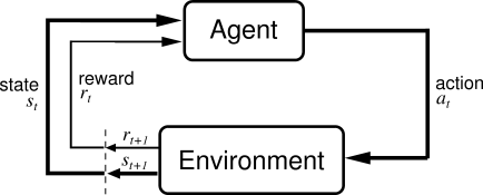
One of the indispensable part of any RL algorithm would be the sampling, where the agent, represented by the policy network in this case, actually interacts with the environment as per Figure 1. More specifically, in the DDPG algorithm, we alternate between the (1) policy sampling and the (2) policy update phase until we obtain an agent that can solve the task (sometimes it just can’t though, unfortunately).
The one we are interested in this section is obviously the (1) policy sampling phase, se already setup the environment earlier.
While the agent interacts with the environment, we need to store the various transitions that will be consequently formed in what can be thought of as the memory of the agent.
We use the previously imported SimpleReplayBuffer class to instantiate the said “memory” component.
buffer = SimpleReplayBuffer( env.observation_space, env.action_space, args.buffer_size, args.batch_size)
Following this, we enter the training loop itself, which namely consists of having the agent interact with the environment (sampling), then update its weight so it performs better, alternatively.
## A few variables to track some training stats
global_step = 0 # How many steps has the agent done so far.
global_update_iter = 0 # How many weights update did we do so far.
global_episode = 0 # How many episodes has the agent completed so far.

while global_step < args.total_steps:
  ## Reset the environment to the starting position
  obs = np.array(env.reset())
  done = False

  # Some variable to keep track of the episode return and length
  train_episode_return = 0.
  train_episode_length = 0

  # Sample a full episode
  for _ in range(args.episode_length):

    # At the very beginning, we instead randomly samples action instead of using the policy.
    # This allows the agent to get a better exposure to the dynamics of the environment before actually
    # starting to interact with it.
    if global_step < args.start_steps:
      # Sampling uniformly from the action space
      action = env.action_space.sample()

    else:
      with th.no_grad():
        action = policy.forward([obs]).tolist()[0] # Use the neural network to sample the actions

      action += noise_fn() # Add the noise for exploration
      action = np.clip( action, -act_limit, act_limit) # Make sure the actions are still in the proper range

    next_obs, rew, done, _ = env.step(action) # Apply the action in the environment
    next_obs = np.array(next_obs)

    buffer.add_transition(obs,action,rew,done,next_obs) # Save the transition to the memory (exprience buffer)

    obs = next_obs

    # Tracking the training statisitics
    global_step += 1
    train_episode_return += rew
    train_episode_length += 1

    ##### Updating the policy and q networks #####
    if global_step >= args.start_steps: # Once we have enough data in the buffer.

      for update_iteration in range(args.updates_per_step):
        global_update_iter += 1

        # Sample random transitions from the exprience buffer.
        observation_batch, action_batch, reward_batch, \
                    terminals_batch, next_observation_batch = buffer.sample(args.batch_size)

        # Q function losses and update
        with th.no_grad():
          next_mus = policy_target.forward( next_observation_batch) # sample action with respect to the next observation

          # Compute the target to be used to update the Q Value network
          q_backup = th.Tensor(reward_batch).to(device) + \
              (1 - th.Tensor(terminals_batch).to(device)) * args.gamma * \
              qf_target.forward( next_observation_batch, next_mus).view(-1)

        # Sample the current estimate of the Q Value.
        q_values = qf.forward( observation_batch, action_batch).view(-1)

        q_loss = mse_loss_fn( q_values, q_backup) # Equation 5
        # Mean Square Error between the target network and the current estimate:
        # By minimizing the error that occurs when our current Q Value network
        # outputs estimates, we get better and better accuracy as we do the updates

        # The Optimizer component provided by Pytorch automatically computes the gradient
        # for each weight when calling the `backward()` function.
        q_optimizer.zero_grad()
        q_loss.backward()
        q_optimizer.step() # Actually update the weights as per Equation (6)

        # Next, we update the policy network
        resampled_mus = policy.forward( observation_batch) # Get the current `optimal` actions
        q_mus = qf.forward( observation_batch, resampled_mus).view(-1) # Evaluate how good they are

        # Our original objective is to be maximized. However, PyTorch's
        # AdamOptimizer considers whatever objective function it is fed with to be minimized!
        # Fortunately, we can transform our original, maximization objective
        # into a minimization objective by simply multiplying by -1.
        policy_loss = - q_mus.mean() # Equation 2

        p_optimizer.zero_grad()
        # Computes the gradient of each weight ( or in other words, their respective contribution to our estimate q_mus of how good the actions are)
        policy_loss.backward()
        p_optimizer.step() # Again, actually update the weights of the neural network as per Equation 3

        # Slowly updating the target networks
        if global_update_iter > 0 and global_update_iter % args.target_update_interval == 0:
            update_target_network(qf, qf_target, args.tau)
            update_target_network(policy, policy_target, args.tau)


      # Logging the training statisitics, namely the losses
      if not args.notb:
        train_stats = {
          "q_loss": q_loss.item(),
          "policy_loss": policy_loss.item()
        }
        tblogger.log_stats( train_stats, global_step, "train")
    #### End of update section ###################

    if done:
      global_episode += 1

      # Again. some other stat. logging
      if not args.notb:
        eval_stats = {
          "train_episode_return": train_episode_return,
          "train_episode_length": train_episode_length,
          "global_episode": global_episode
        }
        tblogger.log_stats(eval_stats, global_step, "eval")

      #  We also output something to the terminal
      if global_step >= args.start_steps:
        print("Episode %d -- Tot. Steps: %d -- PLoss: %.6f -- QLoss: %.6f -- Train Return: %.6f"
          % (global_episode, global_step, policy_loss.item(), q_loss.item(), train_episode_return))

      break;

# When reached, the training is basically done. We then clean up.
if not args.notb:
    tblogger.close()
env.close()
This concludes a really basic implementation of the DDPG algorithm.
An important thing to note, however, is that we implemented a few more “tricks” for the experiments, namely:
- More complex exploration startegies such as the Ornstein Uhlenbeck noise process, and the Adaptive Parameter Space Noise[11].
- Target noise smoothing, which consists in also applying some noise method to the actions sampled based on the
next observations, which are used to compute the target for the Q-Value network - Support for multiple Q-Value network functions, which is mainly inspired by the Twin Delayed DDPG ([5])(Pending at the time of writing). This is used to empirically investigate the reduction of the overestimation bias by using multiple Q-Value network. A potential future experiment would be to train multiple different Q-Value networks over different subsets of the state-action space and use their average as the Q-Value network used to update the policy network itself.
- Normalization for the policy and Q-Value network’s network layers. In some yet to determine conditions, layer normalization seems to drastically improve the value learned by the Q-Value network and helps achieve better performance than the standard neural network, especially in complex environments.
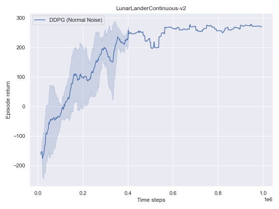
Experiments and Results
We first start with some basic continuous action environments namely Pendulum-v0, InvertedPendulum-v0, and MountainCarContinuous-v0 of the OpenAI Gym basic environments.
Default Settings: Results
Here, we investigate how well a basic implementation of the DDPG algorithm fares on toy problems, namely the Pendulum-v0 and the MountainCarContinuous-v0, which are considered toy problems for RL agents.
Toy problems
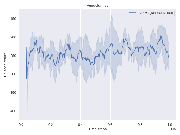
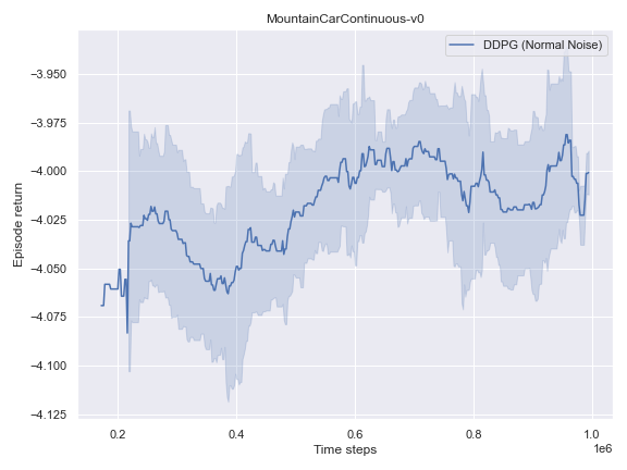
Overall, DDPG seems to solve 2 out of 3 tasks with the default configuration. While it struggles to make consistent progress on MountainCarContinuous-v0, it is still possible to learn a policy that solves the task with an appropriate noise method in this section.
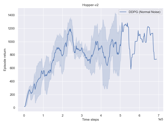
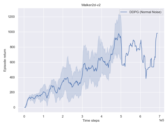
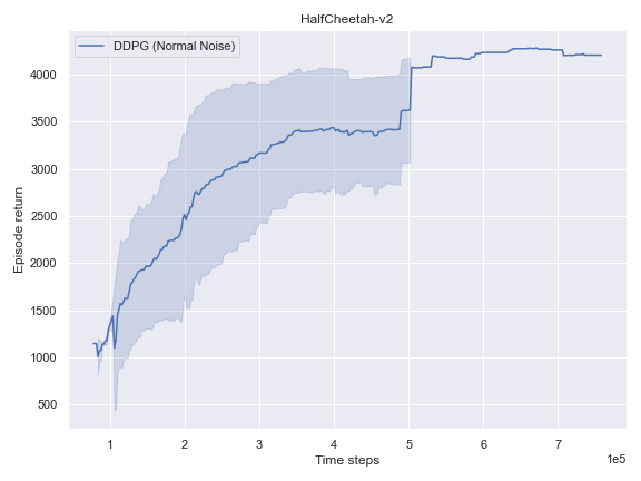
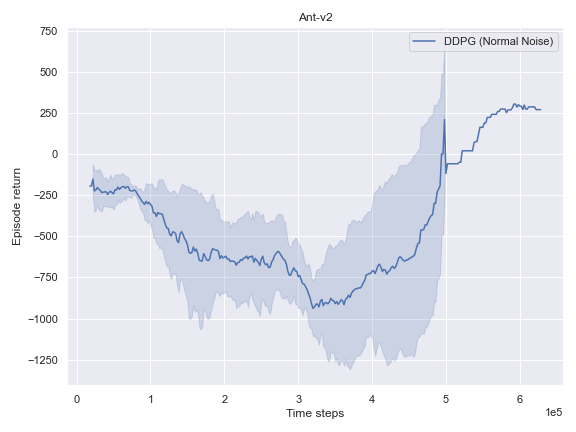
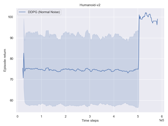
Mujoco
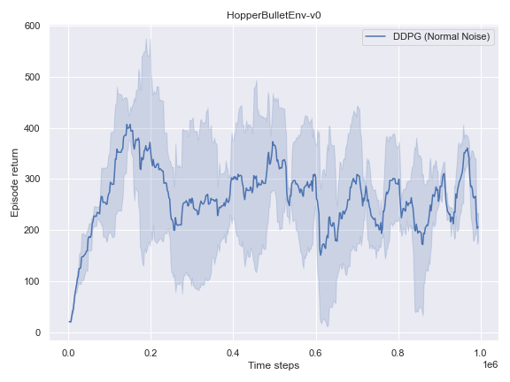
BulletEnv
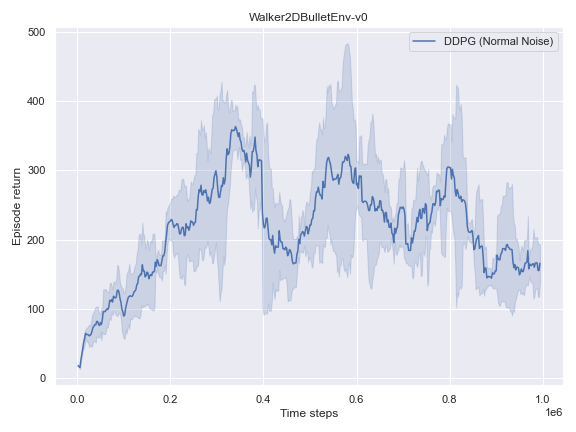
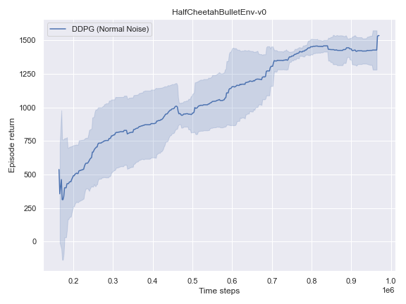
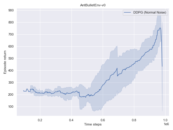
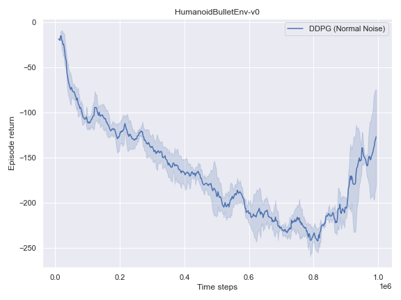
The complete logs data and plots can be accessed and interacted freely with at the following WANDB Report.
Empirical investigation of the noise method
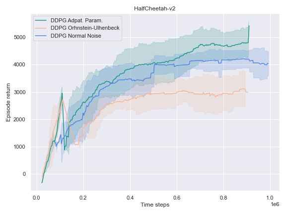
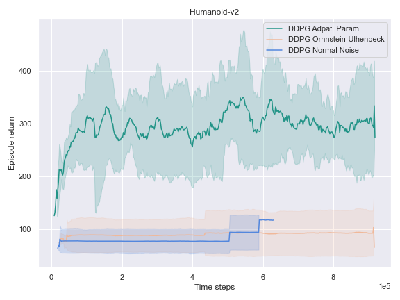
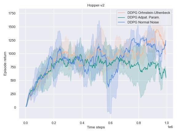
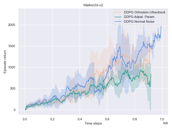
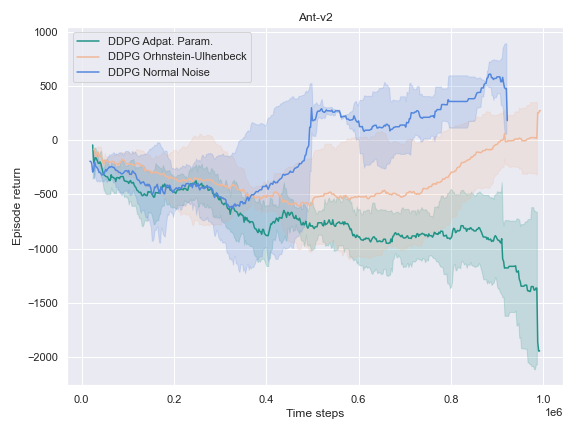
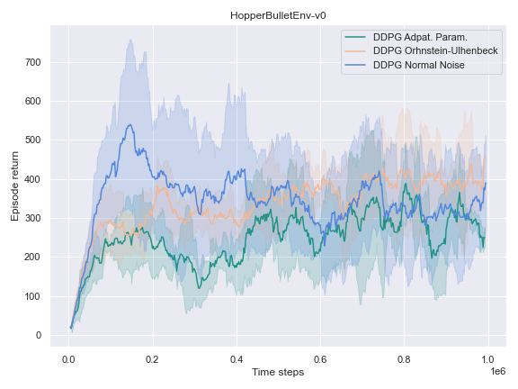
The success of the DDPG algorithm could be said to be closely tied to the effectiveness of the exploratory method. After all, if the agent is not exposed to the parts of the state-action space which leads to the final goal, it is unlikely that it will improve either its Q-value function estimate, or its policy. Therefore, we settle to investigate the impact of different noise methods and their impact on the performance of their policy. Namely, the focus was placed on the following 3 noise functions:
- The default noise sampled from a Normal distribution of zero mean and $0.2$ standard deviation.
- The Ornstein Ulhenbeck noise process Ornstein[12], which, intuitively, sample a noise that is correlated through time.
- The Adaptive Parameter Space noise method [11].
Following this method, the exploration is taken care of by perturbing the parameters of the policy network used for sampling, instead of adding the noise to the output action.
This is indeed desirable, as the exploration policy is made to be state-dependent.
It is further touched upon in the section State-dependent exploration of the paper, namely as follows:
… there is a crucial difference between action space noise and parameter space noise. Consider the continuous action space case. When using Gaussian action noise, actions are sampled according to some stochastic policy, generating $a_t = \pi(s_t) + \mathcal{N} (0, \sigma^22 I)$. Therefore, even for a fixed state $s$, we will almost certainly obtain a different action whenever that state is sampled again in the rollout, since action space noise is completely independent of the current state $s_t$ (notice that this is equally true for correlated action space noise). In contrast, if the parameters of the policy are perturbed at the beginning of each episode, we get $a_t = \pi(s_t)$. In this case, the same action will be taken every time the same state $s_t$ is sampled in the rollout. This ensures consistency in actions, and directly introduces a dependence between the state and the exploratory action taken.
It could hardly be explained better. It indeed turns out to be very useful to learn a good policy, especially in the harder tasks that could not be solved by the vanilla version of DDPG.
Dramatical improvements could be noticed in the case of the MountainCarContinuous-v0 environment, as per the graph and video below:

This phenomenon also occurred for the HalfCheetah-v2 and Humanoid-v2environments.
On the other environments, however, the Adaptive Parameter Space Noise method performed equivalently to the other methods.
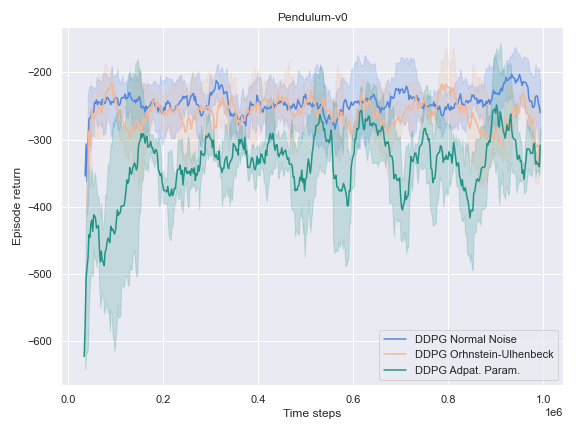
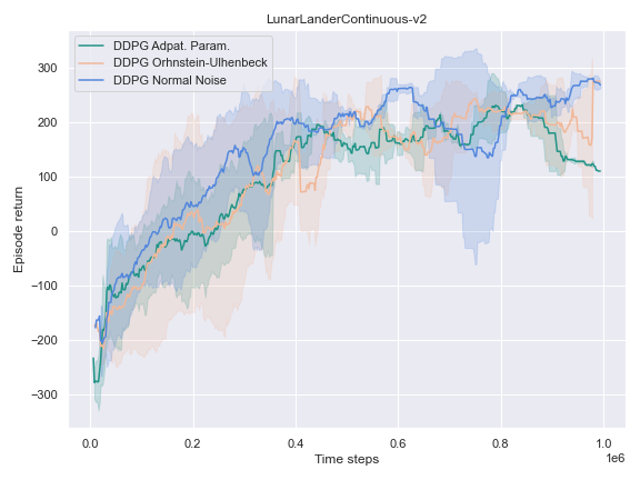
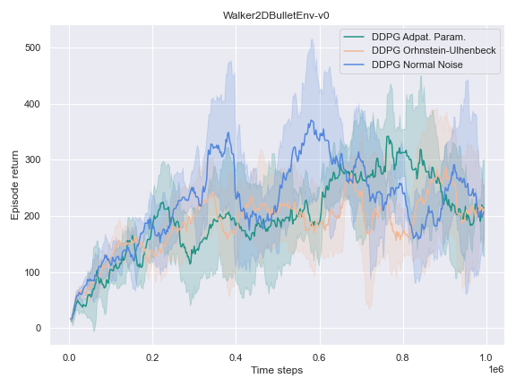
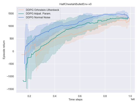
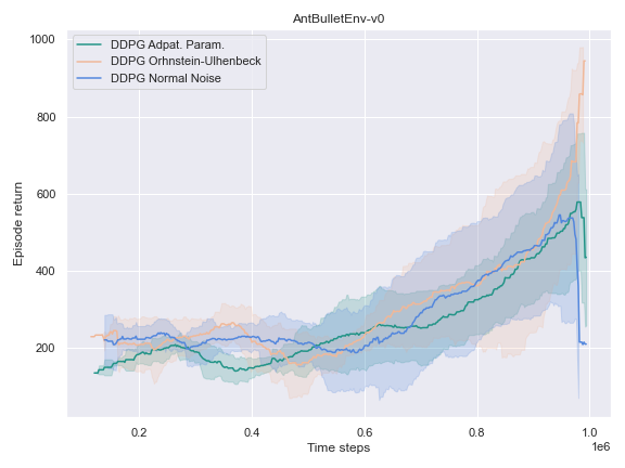
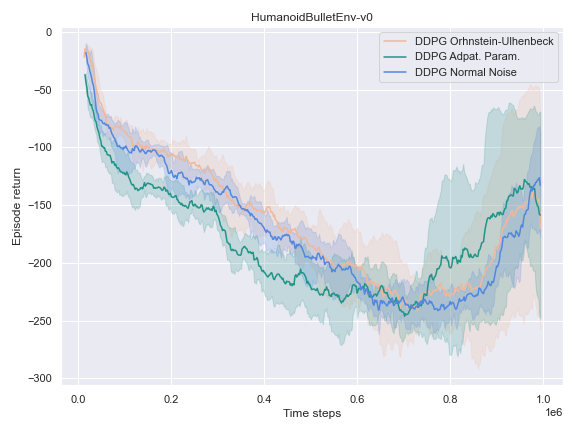
This could use a deeper analysis of the results, the hyperparameters used, as well as the source code for potential wrongdoings, as the original paper boasts improvements on most of the tasks it was experimented on.
Coming Next
- Investigation of the impact of the starting steps hyperparameter. This defines how many steps are randomly sampled before the various networks are updated. Once that threshold is exceeded, the policy of the agent also takes charge of the exploration more actively. While it might not seem that importance of a hyperparameter, turns out it can have a drastic influence on the learning efficiency of the agent, as well as it’s final performance. It seems to be especially relevant in domains such as the Atari 2600 games.
- Layer normalization for the value and policy networks. This technique is advertised as an improvement orthogonal to the machine learning algorithm used. In some experiments, it indeed improved the performance of the agent drastically, especially when applied to the value functions. Further empirical investigation should lead to potentially useful insights. Layer normalization is also a crucial component when using the Adaptive Parameter Space noise method.
- Building toward the TD3 algorithm, it might be interesting to investigate the respective impact of the use of target networks action smoothing, as well as more the impact of having more than one Q-value function estimator.
Acknowledgment
- CleanRL library for a cleaner structure of the source code.
- OpenAI Baselines for all the noise helper functions, as well as the implementation logic of the Adaptive Parameter Space noise method.
Leave a comment