
Soft Actor-Critic: Re-Implementation and Experiments
Foreword
After holding on to this post for almost two years and a half, I decided to just post it as it is and maybe do some updates if needs be. In retrospect, I had what I thought of as quite a few ambitious plans for the reproduction and additional experimentation plans on hyperparameters, tasks, and implementation details of SAC, but alas, due to limitations in time and computation resources, I had to leave it at the current content. For a more succinct write-up on SAC implementation, I would recommend CleanRL’s SAC documentation page which goes straight to the point.
Some of the things I wanted to explore but did not have the time to do would be:
-
A more comprehensive investigation of the impact of the automatic entropy tuning and its influence and the policy and soft q-value networks losses, as well as the exploration of the policy itself.
-
The impact of using this or that policy structure, as described in the relevant section, but the reproduction effort was non-negligible (neural network architecture, activation functions, and the parameterization scheme of the action distribution of the policy). Furthermore, some later experience in the field of machine learning, neural network training, and reinforcement learning made it intuit that unlike PPO’s implementation details the implementation details of the policy were not that important for the already robust SAC algorithm. It did not seem that there would be any meaningful improvement over the baseline after all.
-
A more comprehensive investigation of the impact of the update regime for the Q-value networks as well as the policy. For example, if we follow TD3’s logic, the policy is updated every two Q-value network updates. The rationale behind this was that using a more accurate, or in other words, more updated Q-value network would lead to a better and more stable policy.
In the end, the investigation of these implementation details did not seem like a worthy pursuit, as time went by. This post is thus more about getting closure so that I can finally start writing on deep RL algorithms that are more recent and relevant to my research.
Introduction
The Soft Actor Critic (SAC) ([1], [2], [3], [4], [5]) is built on top of the various progress made in Deep Reinforcement Learning (DRL) for continuous control. It happens to address some of the shortcomings of the Deep Deterministic Policy Gradient (DDPG) ([6]) method. Since the SAC algorithm is strongly related to the latter, being familiar with it should greatly facilitate understanding the SAC algorithm itself. (For the sake of completeness, a similar write-up for the DDPG algorithm and some of its intricacies can be found here.)
As an outline, we first attempt at introducing the theory behind SAC in an intuitive way. Then, we go over the various implementation details of SAC that can be found across the various publicly available implementations, then introduce our reimplementation, based on the workflow of the CleanRL Reinforcement Learning library. Additionally, we present some results of training an SAC agent over some popular DRL environments, as well as some additional experiments that we thought would be interesting to play around with.
Without further ado, let us start with an overview before diving into the nitty-gritty details of the aforementioned algorithm.
Background
Reinforcement Learning
Reinforcement Learning (RL) is usually approached through the lenses of the Markov Decision Process (MDP), in the most straightforward cases. The MDP is defined as a five-tuple \((S,A,P(s'\vert s, a),R(s,a),\gamma)\), which respectively stand for the state space, action space, transition dynamics, reward function and discount factor (more here).
The objective of a standard RL agent \(\pi\) is to maximize the expected future reward denoted here as \(J\), which can be formally defined as:
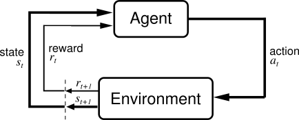
\[J_\pi = \mathbb{E}_{s_t \sim P(\cdot \vert s_{t-1}, a_{t-1}), a_t \sim \pi(\cdot \vert s_t)} \left[ \sum_{t=0}^{\infty} \gamma ^ t r(s_t,a_t)\right] \quad (1)\]The agent is expected to achieve such a goal through a trial-and-error process of interacting with the environment (Figure 1) and collecting experience (also referred to as sampled trajectories, formally written as the tuple (s, a,r,s’)).
Deterministic Policy Gradient
From personal experience, before challenging the SAC algorithm, it might be useful to get familiar with the simpler but shared structure of offline policy gradients methods such as the DDPG (OpenAI SpinningUp’s DDPG). This is motivated by the observation that the key differences between DDPG and SAC are:
- (1) a stochastic policy (which is also related to the entropy maximization aspect)
- (2) having two Q-networks.
Key components of the SAC algorithm
1. Entropy Maximization
As a direct consequence of having a stochastic policy, an additional reward derived from the entropy maximization objective can be added on top of the environment’s reward. Intuitively, when we have a low entropy policy, the actions it outputs in a given state are consistent, or in other words, have low variance. For example, a deterministic policy such as in DDPG has an entropy of 0, since, for any given state, the same action will be output by the policy network every time it is queried.
A moderate to high entropy policy, on the other hand, when given the same state, would instead output a different action every time we sample from it. The higher the distance between the actions, the higher the entropy. As described in the sub-section above, such high entropy policy implicitly incorporates some exploratory noise, which is also dependent on the current state.
The entropy maximization objective is formally expressed by adding the entropy of the policy, weighted by the scalar $\alpha$ in the original Equation (1), thus yielding the entropy maximization objective:
\[J_{\pi}^{\mathrm{MaxEnt}} = \mathbb{E}_{ (s_t,a_t) \sim \rho_{\pi}} \left[ \sum_{t=0}^{\infty} \gamma ^ t r(s_t,a_t) + \alpha \mathcal{H}\left[\pi(\cdot \vert s_t) \right] \right] \quad (2)\]where \(\rho_{\pi}\) represets the state-actions transitions (or \((s,a)\) trajectories basically) that are induced by following said policy \(\pi\).
2. Stochastic Policy:
In contrast with the DDPG, which is built on top of a deterministic policy, the SAC algorithm instead leverages a parameterized stochastic policy, which happens to be more expressive than its deterministic counterpart. Namely, a stochastic policy can allow the agent to capture multiple near-optimal policies in the same structure. An example of where this comes in handy could be described as follows: let us imagine the context of an agent controlling a car, that tries to go from city A to city B. Now there might be multiple roads that lead from A to B, and since we want the agent to get there as fast as possible, we are interested in the short path. There might exist two different roads that have the same, shortest length. A deterministic agent would only be able to capture a single one of them (this is assuming it can first find it), while a stochastic agent would be able to capture both of the roads. While this is a simplistic example, this is an invaluable property when we need the agent to be able to achieve some arbitrary goal in different ways.
The second benefit of having a stochastic policy would be state-dependent exploration. Considering the actions being sampled from a Normal distribution parameterized by the mean and the standard deviation. The mean action could be considered as the deterministic action the deterministic policy would take, such as in DDPG. The standard deviation allows us to define a neighborhood around said mean action, such that actions that “are not necessarily the best” also get sampled from time to time.

Therefore, by conditioning the standard deviation parameter of our Normal distribution on the state $s$, the agent can implicitly learn to control how much exploration (how far away from the “current” optimal action) to apply while interacting with the environment. Intuitively, the standard deviation of the agent for a state that it has encountered often enough would become lower as the agent converges to the optimal action. On the other hand, the standard deviation of the agent for a state that was not seen much before would be high. This in turn will make the agent behave less conservatively around that state, thereby making it explore more, ideally leading it to exhaust the state-action space.
An additional benefit of having a state-dependent exploration is that it also results in a more smooth, correlated exploration process. Indeed, when sampling noise from a normal distribution to add it to an action, for the same state, we would always get different and uncorrelated noise values (see [8]). Parameterizing the “noise” of exploration by conditioning on the state results in more consistent exploratory behavior.
For the sake of completeness, we now formally introduce the notation of the parameterized policy, as well as the derivation of the gradients of said parameters concerning the agent’s objective function. One might however skip this part at first if he is already familiar with the DRL definition, or if he or she does not mind just getting a more abstract picture of the algorithm.
The stochastic policy of the agent is denoted as \(\pi_{\theta}(a \vert s)\), which actually represents a Normal distribution with mean $\mu_{\theta}(s)$ and standard deviation $\sigma_{\theta}(s)$ such that:
\[a \sim \mathcal{N}( \mu_{\theta}(s), \sigma_{\theta}(s))\]Overloading \(J_{\pi}\) with the entropy maximization objective introduced in Equation (2), we aim at training an agent that maximizes said \(J_{\pi}\). Formally, we write:
\[\theta^* = \mathrm{argmax}_{\theta} \enspace J_{\pi}\]The optimization process itself consists in incrementally changing the parameters $\theta$ of the policy network to maximize the probability of actions that contribute to higher rewards while minimizing the probability of those that lead to low rewards. The entropy maximization objective, on the other hand, will impact the policy network parameters so that the actions sampled based on arbitrary states differ as much as possible, while still achieving high rewards. Intuitively, this is equivalent to having a policy that will produce different actions for the same state, but the variance of said actions will ultimately be bounded to an interval that still allows the agent to achieve high returns on the task.
In any case, a slightly more practical approach to the objective of the agent is presented here.
3. Soft Q Value function:
As a consequence of introducing the entropy maximization objective, the critic component of the standard actor-critic framework is also impacted. Namely, we now use a Soft Q value function (originally presented back in [1]), which incorporates the entropy component of the policy while estimating the expected discounted future return.
The author posits that the standard value function that evaluates a state-action pair and its corresponding entropy is an implicit policy. Namely, by exponentiating the Q-value of all the actions given an arbitrary state, and regularizing it using the partition function over said state-action space, we can recover a probability distribution over the continuous action space. An intuitive attempt at illustrating this concept is presented in the figure below.

This implicit policy can then be used as a target for the actor’s parameterized policy to optimize against. This process was formally defined as minimizing the KL divergence between the implicit policy recovered from the Soft Q Value and the actor’s policy:
\(J_{\pi}(\theta) = \mathbb{E}_{s_t \sim \mathcal{D}} \Big[ \text{D}_{\text{KL}} \big( \pi_\theta(s_t) \vert \vert \frac{exp(Q_\phi(s_t, \cdot))}{Z_\phi(s_t)} \big) \Big]\) (See [2], Equatin 10).
While it might sound complicated at first, the actual implementation does not differ from the DDPG Q value function Namely, a lot of those operations (exponentiation of the Q value, regularization with partition function, and minimizing the KL divergence between the two policies) happen to simplify themselves later on.
4. Reducing Overestimation Bias with multiple critic functions
This implementation component seems to have been introduced concurrently by not only the SAC algorithm but also the Twin Delayed Deep Deterministic Policy Gradient (abbreviated as TD3 [7]) (at least when it comes to the continuous action space case). (If we refer to the order in which the arXiv preprints were published, it might seem that the SAC [2] implements it first. However, the TD3 paper explicitly investigates the problem of overestimation bias that occurs in DDPG, which suggests it is the origin of the technique of using multiple Q value functions).
Over-estimation bias can be understood as the Q function (or analog component) being overly optimistic, and consequently misrepresenting the landscape of the state-action space in which the agent’s policy makes its decision. Let us recall that in the policy gradient method, we aim at maximizing the likelihood of the actions that bring the agent the most reward, namely by following the guidance of the Q value function. However, the Q value function itself is trained on trajectories data that are sampled with a sub-optimal policy. If the latter does not output actions that are close to the optimal ones for a given state, the Q value function is likely to attribute a higher value to those actions that are sub-optimal, to the detriment of the optimal actions. Hence, the Q-value function overestimates the value of an action given an arbitrary state.
To mitigate this, the concept of using the minimum of at least 2, or more generally, an ensemble of Q-values functions were introduced. Intuitively, since the output of each respective Q-value function is bound to be different, by taking the minimum of the estimated values of each action, we end up with a more conservative, and less biased approximation of its actual value. This in turn dramatically increases the performance and learning stability of the agent, as demonstrated in [7]).
Implementation details
This write-up compiles various implementations methods that appear across popular reinforcement learning libraries/repositories, as well as a few of the lesser-known ones, namely:
- Original implementation by Tuomas Haarnoja et al. (Tensorflow v1.4) Link
- Stable Baselines (Tensorflow 1.XX) Link
- OpenAI Spinning Up (Tensorflow 1.XX, then later in PyTorch) Link
- Denis Yarats and Ilya Kostrikov’s Implementation (Pytorch) Link
The component that happens to have the most variance in all those implementations happens to be the policy, which we go over in the next section.
Policy network
Given the implementations mentioned above not only use different deep learning frameworks but also adopt different structuration, we attempt to approach their respective implementations from a high-level (pseudo code) perspective, we focus on the flow of the mapping from the observation received by the environment to the action distribution.
First, an high-level overview of the various policy structure encountered is summarized in the graph below.
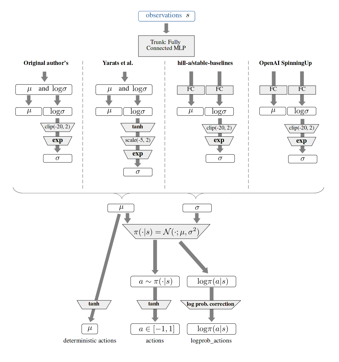
A more detailed, while deep learning framework-agnostic overview of those different implementations’ respective pseudo-code can be found further down below (Appendices).
Policy network implementation differences A summary of the core difference between those implementations is as follows:
- Either “Joint or disjoint parameterization” of the mean $\mu$ and log standard deviation $log \sigma$.
- Clipping or shifting the range of the $log \sigma$
- L2 regularization of the policy network’s weights
- Squashing of the action with the $tanh$ function, and adjusting the $log\pi(a \vert s)$ correspondingly.
While the main difference in those implementations is the way the action distributions are parameterized (especially $\mathrm{log}\sigma$), their respective behaviors end up being similar, as per the following interactive graph that modelizes the respective distributions.
Hyper-parameters
Additionally, we have taken this opportunity to summarize the various hyper-parameter values used across the repositories referenced above for more convenient comparison.
| Hyperparameter | Haarnoja et al. | Stable Baselines | SpinningUp | Yarats et al.’s |
|---|---|---|---|---|
| General | ||||
| Discount \(\gamma\) | 0.99 | 0.99 | 0.99 | 0.99 |
| Initial exploration (g) | 1000 (a) | 0 (random_exploration) |
10000 (start_steps) |
5000 (num_seed_steps) |
| Tau (target update coef.) | 0.005 | 0.005 | 0.005 | 0.005 |
| Reward scaling | Yes (b) | No | No | No |
| Buffer size | 1e6 | 5e5 | 1e6 | 1e6 |
| Batch size | 256 | 64 | 100 | 1024 |
| Seeding | {1,…,5} | Random by default | 0 by default | 1 by default |
| Entropy coefficient | 0.0 | Auto | 0.2 | 0.1 |
| Entropy auto-tuning | No (c) | Yes, see above | No | Yes |
| Learning starts (g) | 1000 (a) | 100 (learning_starts) |
1000 (update_after) |
5000 (num_seed_steps) |
| Policy | ||||
| Hidden layer dim. | 256,256 | 64,64 | 256,256 | 1024,1024 |
Logstd range clip |
[-20,2] Clip (d) | [-20,2] Clip | [-20,2] Clip | tanh, then scale within [-5,2] |
| Squashing | Yes | Yes | Yes | Yes |
| Update frequency | 1 | 1 | 50 (f) | 1 |
| Learning rate | 3e-4 | 3e-4 | 1e-3 | 1e-4 |
| Activation | ReLU (e) | ReLU | ReLU | ReLU |
| Weight, Bias init. | Xavier, Zeros | Xavier, Zeros | Torch nn.Linear’s default | Torch nn.Linear’s default |
| Soft Q-Networks | ||||
| Hidden layer dim | 256,256 | 64,64 | 256, 256 | 1024,1024 |
| Learning rate | 3e-4 | 3e-4 | 1e-3 | 1e-4 |
| Update frequency | 1 | 1 | 50 (f) | 2 |
| Activation | ReLU (e) | ReLU | ReLU | ReLU |
| Weight, Bias init. | Xavier, Zeros | Xavier, Zeros | Torch nn.Linear’s default | Torch nn.Linear’s default |
Some additional notes regarding the hyper-parameters, or more general components of the implementations:
- (a) Some hyperparameters were set according to the specific environment, see here.
- (b) Also varies depending on the environment. The method of determination does not seem to be provided, however. Probably some “human priors”: Link.
- (c) Added later in another repository, more specifically here
- (d) While some implementations (Haarnoja et al., Stable Baselines, SpinningUp, directly clip the
logstdto the bounding interval ([-20, 2]), Yarats et al first appliestanhthen scale it to the interval[-20,2]. - (e) The source codes also includes the option to use the
tanhnon-linear activation, but the difference is result does not seem to be explored. - (f) In OpenAI SpinningUP, the network updates are not done at every time step, but in an “epoch-based” fashion. Namely, a specific amount of transitions are collected, before updating the policy and critic network. In other words, the “sample-update” regime is different. There is not much difference in the empirical result, however.
- (g) The concept of
Initial explorationandLearning startscan be found across various implementations, not limited to the SAC algorithm. The former is consistently used (DQN, DDPG, etc…) and determines how many steps are sampled using a uniform or random distribution over the action space, to fill the agent’s experience with diverse, “non-biased” trajectories. This is done to learn an accurate enough critic function at the beginning of the training, to provide a less biased, and thus better feedback to the policy once it starts to learn. TheLearning Startshyperparameter is less common and determines after how many steps we start updating the networks. Intuitively, this also makes sure we have enough data in the replay buffer before starting the updates. From personal experience, this hyper-parameter hardly had mostly no impact on continuous control toy problems and Mujoco locomotions tasks. - The original author’s implementation, as well the one from OpenAI SpinUp evaluates the agent’s performance using a deterministic policy, i.e. the mean of the action. Some argue, however, that being an entropy maximization method among other things, SAC agents should still be evaluated in the stochastic mode to exhibit the whole range of diversity learned by the policy.
Besides the implementation details touched upon above, the other aspects of the SAC algorithm implementation are essentially the same across repositories. From here onward, we go over a simplified implementation of the aforementioned components with the technique that worked best during our re-implementation phase.
Simplified implementation
Soft Q-Value function
The Soft Q-Value is likely the component with less variance across the various reference implementation. Similar to DDPG [6], the Q value function simply maps from the concatenation of the current state and the action $s || a$ to a real value.
Hereafter is a snippet of a simple implementation of such a network using the Pytorch Deep Learning framework.
# observation_shape: the dimension of the observation vector that serves as input to the network
# action_shape: the dimension of the action vector

class SoftQNetwork(nn.Module):
    def __init__(self):
        super(SoftQNetwork, self).__init__()
        self.fc1 = nn.Linear(observation_shape+action_shape, 256)
        self.fc2 = nn.Linear(256, 128)
        self.fc3 = nn.Linear(128, 1)

    def forward(self, x, a):
        x = torch.Tensor(x).to(device)
        x = torch.cat([x, a], 1)
        x = F.relu(self.fc1(x))
        x = F.relu(self.fc2(x))
        x = self.fc3(x)
        return x
The same, but more contextualized implementation can be found in the SAC implementation of the CleanRL library.
Soft Q-Network objective and optimization
Slightly different from the traditional Q-network objective (DDPG, TD3, etc…), which predicts the “pure” expected discounted future return given a state, the Soft Q-Network incorporates the entropy of the policy into its objective, namely:
\[Q^{\pi}(s,a) = \mathbb{E}_{s' \sim P,a' \sim \pi} \big[ R(s,a) + \gamma (Q^\pi(s',a') + \alpha \underbrace{\mathcal{H}(\pi(\cdot \vert s'))}_{\text{policy's entropy}}) \big]\](A more in-depth explanation is provided in OpenAI SpinningUp, and / or the author’s definition in Eq. 3)
The training objective of the Soft Q-Networks thus consists in reducing the soft Bellman residual as follows:
\[J_{Q}(\theta) = \frac{1}{2} \mathbb{E}_{(s_t, a_t, r_t, s_{t+1}) \sim \mathcal{D}} \Big[ (Q_\theta(s_t, a_t) - y)^2 \Big] \\ \text{with} \enspace y = r(s_t, a_t) + \gamma (Q_\theta(s_{t+1},a_{t+1}) - \alpha \text{log} \pi_{\phi}(a_{t+1} \vert s_{t+1})), \\ \text{and where} \enspace a_{t+1} \sim \pi_\phi(\cdot \vert s_{t+1}),\]where $(s_t,a_t,r_t,s_{t+1} \sim \mathcal{D})$ represent a batch of state, action, reward and next_state sample from the agent’s experience (trajectories collected by having the agent’s policy $\pi_{\phi}$ interact with the environment).
The mitigation of the over-estimation bias argued for in the original paper is thus achieved by having two (or more) independently parameterized soft Q-networks. Be it in the SAC, or the TD3 algorithm, the number of Q-network required to do so was empirically determined to be “at least 2”
In any case, letting our two soft Q-networks be $Q_{\theta_1}$ and $Q_{\theta_2}$ respectively parameterized by $\theta_1$ and $\theta_2$, the more explicit optimization objective can be written as follows:
\[J_{Q}(\theta_{i}) = \frac{1}{2} \mathbb{E}_{(s_t, a_t, r_t, s_{t+1}) \sim \mathcal{D}} \Big[ (Q_{\theta_i}(s_t, a_t) - y)^2 \Big] \\ \text{with} \enspace y = r(s_t, a_t) + \gamma ({\color{red} \min_{\theta_{1,2}}Q_{\theta_i}(s_{t+1},a_{t+1})} - \alpha \text{log} \pi_{\phi}(a_{t+1} \vert s_{t+1}))\]Practically speaking, this whole optimization of the Soft Q-Networks is achieved by the following snippet of code:
# sample data from agent's experience
s_obs, s_actions, s_rewards, s_next_obses, s_dones = rb.sample(args.batch_size)

with torch.no_grad():
    # get next action a_{t+1} and log pi(a_{t+1} | s_{t+1})
    next_state_actions, next_state_log_pi, _ = pg.get_action(s_next_obses, device)
    # get Q_1(s_{t+1}, a_{t+1})
    qf1_next_target = qf1_target.forward(s_next_obses, next_state_actions, device)
    qf2_next_target = qf2_target.forward(s_next_obses, next_state_actions, device)

    # add the minimum of the Q values and add the policy entropy bonus
    min_qf_next_target = torch.min(qf1_next_target, qf2_next_target) - alpha * next_state_log_pi

     # this is the y in the equations above.
    next_q_value = torch.Tensor(s_rewards).to(device) + \
        (1 - torch.Tensor(s_dones).to(device)) * args.gamma * (min_qf_next_target).view(-1)

# get Q_1(s_t, a_t)  and Q_2(s_t, a_t)
qf1_a_values = qf1.forward(s_obs, torch.Tensor(s_actions).to(device), device).view(-1)
qf2_a_values = qf2.forward(s_obs, torch.Tensor(s_actions).to(device), device).view(-1)

# Compute the TD error with respect to y(s,a) for the Q networks
qf1_loss = loss_fn(qf1_a_values, next_q_value)
qf2_loss = loss_fn(qf2_a_values, next_q_value)
qf_loss = (qf1_loss + qf2_loss) / 2

# here, values_optimizer is an Adam (torch.optim.Adam) optimizer that applies stochastic gradient
values_optimizer.zero_grad()
qf_loss.backward()
values_optimizer.step()
For the more contextualized source code, please refer to this link.
As a side experiment, the impact of the number of Q-networks was empirically investigated. Besides re-asserting the drastic improvement of having at least 2 Q-network, thus mitigating the overestimation bias, having more than 2 Q-network did not seem to be worth the cost in memory, code complexification, and additional computational cost (at least not in the limited tasks that were experimented on). For the sake of completeness, the results can be accessed here.
Policy network
Finally, we present a snippet of the implementation used, which uses the “disjoint parameterization” method, but the tanh the scaling processing applying to the logstd component.
# observation_shape: the dimension of the observation vector that serves as input to the network
# action_shape: the dimension of the action vector
# LOG_STD_MAX = 2
# LOG_STD_MIN = -5

class Policy(nn.Module):
    def __init__(self):
        super(Policy, self).__init__()
        self.fc1 = nn.Linear(observation_shape, 256) # Better result with slightly wider networks.
        self.fc2 = nn.Linear(256, 128)
        self.mean = nn.Linear(128, action_shape)
        self.logstd = nn.Linear(128, action_shape)
        # action rescaling
        self.action_scale = torch.FloatTensor(
            (env.action_space.high - env.action_space.low) / 2.)
        self.action_bias = torch.FloatTensor(
            (env.action_space.high + env.action_space.low) / 2.)
        self.apply(layer_init)

    def forward(self, x):
        x = torch.Tensor(x).to(device)

        x = F.relu(self.fc1(x))
        x = F.relu(self.fc2(x))
        mean = self.mean(x)
        log_std = self.logstd(x)
        # From Denis Yarats' implementation: scaling the logstd with tanh,
        # and bounding it to a reasonable interval
        log_std = torch.tanh(log_std)
        log_std = LOG_STD_MIN + 0.5 * (LOG_STD_MAX - LOG_STD_MIN) * (log_std + 1)

        return mean, log_std

    def get_action(self, x):
        mean, log_std = self.forward(x)
        std = log_std.exp()
        normal = Normal(mean, std)
        x_t = normal.rsample()  # reparameterization trick (mean + std * N(0,1))
        y_t = torch.tanh(x_t)
        action = y_t * self.action_scale + self.action_bias
        log_prob = normal.log_prob(x_t)
        # Enforcing Action Bound with tanh squashing
        log_prob -= torch.log(self.action_scale * (1 - y_t.pow(2)) +  1e-6)
        log_prob = log_prob.sum(1, keepdim=True)
        mean = torch.tanh(mean) * self.action_scale + self.action_bias

        return action, log_prob, mean

    def to(self, device):
        self.action_scale = self.action_scale.to(device)
        self.action_bias = self.action_bias.to(device)
        return super(Policy, self).to(device)
Similar to the Q-network, a more contextualized implementation can be found here.
Policy’s objective and optimization
Recall the maximum entropy objective from Eq. 2 our agent is expected to optimize toward. In practice, with a parameterized Gaussian policy $\pi_\phi$ as described above, the objective becomes:
\[\text{max}_{\phi} \, J_{\pi}(\phi) = \mathbb{E}_{s \sim \mathcal{D}} \Big[ \text{min}_{j=1,2} Q_{\theta_j}( s, a) - \alpha \text{log}\pi_{\phi}(a \vert s) \Big] \\ \text{where } a = \mu_{\phi}(s) + \epsilon \, \sigma_{\phi}(s), \text{ with } \epsilon \sim \mathcal{N}(0, 1) \text{ (reparameterization trick.)}\]Intuitively, we optimize the weights $\phi$ of the policy network so that it (1) outputs actions $a$ that correspond to a high Q-value $Q(s, a)$, while at the same time (2) making sure that the distribution over those actions $a$ is random enough (maximum entropy).
This part is quite straightforward to implement, as per the follow code snippet.
# sample data from agent's experience
s_obs, s_actions, s_rewards, s_next_obses, s_dones = rb.sample(args.batch_size)

# get action and their log probability
pi, log_pi, _ = pg.get_action(s_obs, device)

# get Q-value for state action pairs
qf1_pi = qf1.forward(s_obs, pi, device)
qf2_pi = qf2.forward(s_obs, pi, device)
min_qf_pi = torch.min(qf1_pi, qf2_pi).view(-1)

# maximiizes Q(s,a) and -log \pi(a|s), as per Eq. above
policy_loss = ((alpha * log_pi) - min_qf_pi).mean()

# apply one gradient update step
policy_optimizer.zero_grad()
policy_loss.backward()
policy_optimizer.step()
Also, a note on having two optimizers in the SAC
Automatic Entropy tuning
In the objective of the policy defined above, the coefficient of the entropy bonus $\alpha$ is kept fixed all across the training. As suggested by the authors in Section 5 of their Soft Actor-Critic And Applications([4]), the original purpose of augmenting the standard reward with the entropy of the policy is to encourage explorations of yet well enough explored state (thus high entropy). Conversely, for states where the policy has already learned a near-optimal policy, it would be preferable to reduce the entropy bonus of the policy, so that it does not lose its way by exploring, due to being encouraged to have high entropy.
Therefore, having a fixed value for $\alpha$ does not fit this desideratum of matching the entropy bonus with the knowledge of the policy at an arbitrary state during its training.
To mitigate this, the authors proposed a method to dynamically adjust $\alpha$ as the policy is trained. While the theoretical method that is used is skipped for the sake of brevity, the gist would be that they first define an optimization constraint over the reward, subject to a lower bound on the entropy of the policy (the bonus). The optimal value for $\alpha$ happens to be the dual of the optimization problem introduced earlier, which objective is defined as follows:
\[\alpha^{*}_t = \text{argmin}_{\alpha_t} \mathbb{E}_{a_t \sim \pi^{*}_t} \big[ -\alpha_t \, \text{log}\pi^{*}_t(a_t \vert s_t; \alpha_t) - \alpha_t \mathcal{H} \big],\]where \(\mathcal{H}\) represents the target entropy, or in other words, the desired lower bound for the expected entropy of the policy over the trajectory distribution $(s_t, a_t) \sim \rho_\pi$ induced by the latter. As a heuristic for the target entropy, the authors use the dimension of the action space of the task.
Once the optimization problem is formulated this way, the implementation becomes relatively straightforward:
## Before the training actually begins
# defined an initial value for (log) alpha,
# as well as thecorreponding optimizer (Adam)
target_entropy = - torch.prod(torch.Tensor(env.action_space.shape).to(device)).item()
# instead of alpha, uses log_alpha for numerical stability
log_alpha = torch.zeros(1, requires_grad=True, device=device)
alpha = log_alpha.exp().item() # the actual value of alpha
a_optimizer = optim.Adam([log_alpha], lr=1e-3)
With the optimizer declared above, the log_alpha is then updated jointly with the policy as follows, to tweak the value of $\alpha$ based on the current entropy of the policy, as per the equation above.
with th.no_grad():
    _, resampled_logprobs = policy.get_actions(observation_batch)
alpha_loss = (-log_alpha * (resampled_logprobs + target_entropy)).mean()

a_optimizer.zero_grad()
alpha_loss.backward()
a_optimizer.step()

alpha = log_alpha.exp().item()
Experiments
Automatic Entropy Tuning
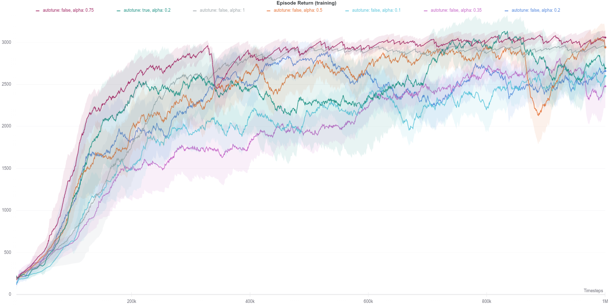
To get a better understanding of how the automatic entropy tuning works, SAC agents were trained using a limited range of \(\alpha\) values, as well as the tuned \(\alpha\) agent was run on a limited set of Mujoco robotic control tasks.
The experiment results themselves can be further interacted with using the following WANDB Report.
TL;DR: Overall, we observed that the best value for the entropy bonus coefficient, \(\alpha\) drastically varies depending on the task. The method proposed to automatically tune said values results in very small values of \(\alpha\) as training progresses. Intuitively, the more the agent trains, the less random we want its policy to b While this method does perform well enough over the task experimented upon, it might be better used as a starting point when applying SAC to a new environment, before performing additional fine-tuning of the \(\alpha\) coefficient itself to achieve better performance.
The conducted analysis on this component of the implementation can be found in the appendix.
Multiple Q-Networks
Earlier in the sub-section 4., we went over how using multiple critics allowed the agent to obtain a more useful approximation of the Q-value function by using at least 2 Q-networks. While the TD3 paper does mention experimenting with more than 2 Q-networks, but for the TD3 algorithm.
The objective of this set of experiments was to also verify the impact of using more than 2 Q-networks for the SAC algorithm.
- First, we can easily observe that using at least 2 Q-networks results in a drastic performance improvement, but also stability of the learning across all tasks.
- While using 2 Q-network does good enough results, some environments did benefit from having more. Namely, having 3 Q-Networks did seem to improve not only the final performance but also the stability and the efficiency of the agent’s learning. This trend can be observed namely on the Hopper-v2, Walker2d-v2, Ant-v2, and Humanoid-v2 (the latter, to a certain extent). It nevertheless incurs an additional computational cost that should be taken into account when running extensive experiments. (Ideally, the Q-network would be run ‘in parallel’).
- Beyond 3 Q-networks, there is hardly any consistent improvement in performance or stability in the performance of the agent. If anything, as the number of Q-network, rises, the performance seems to saturate at sub-optimal levels. As an example, SAC with Number of Q-Networks \(\in {5,8,10}\) performs as, if not worse than when using a single Q-network. Hypothetically, this would be due to an overly conservative Q-value which results in the agent not exploring much, thus converging to a sub-optimal policy.
Policy update delay (following TD3)
This experiment consisted in investigating the impact of the policy update delay mechanism notably introduced in the TD3 paper, and subsequently appearing in other public implementations.
The default practice is to update the policy network every second update of the critic networks (the hyperparameter --actor-update-interval=2, code-wise).
Intuitively, the aim is to update the policy by using the more accurate Q-network.
This is implemented as the snippet below:
## Policy update section: delay the updates by 'actor_update_interval',
## but compensate by also doing 'actor_update_interval' updates to the network
## global_step is the number of interactions with the environment so far
## (also coincides with the number of updates of the Q-networks)
if global_step % args.actor_update_interval == 0:
    for _ in range(args.actor_update_interval):
        resampled_actions, resampled_logprobs = policy.get_actions( observation_batch)

        qf1_pi = qf1(observation_batch, resampled_actions).view(-1)
        qf2_pi = qf2(observation_batch, resampled_actions).view(-1)
        min_qf_pi = th.min(qf1_pi,qf2_pi)

        policy_loss = (alpha * resampled_logprobs - min_qf_pi).mean()

        p_optimizer.zero_grad()
        policy_loss.backward()
        p_optimizer.step()

## ... rest of the training
-
In the experiments conducted, the final performance of the agent does not differ too much across the range of values of the hyperparameter investigated in this section, namely
actor_update_interval\(\in \{1,2,3,5,8\}\). -
However, following the plots (or experiment results) below, updating the policy network with the same frequency as the Q-networks (i.e.
actor-update-interval= $1$) yielded better final performance than the delayed update version withactor-update-interval= $2$. -
As for other values of that hyperparameters, there is no consistent improvement in the agent’s performance across the environments investigated.
The observations above are based on the experimental results summarized in the following WANDB Report.
Conclusion
In this post, we went over the various implementations of the SAC algorithms publicly available. The main difference was identified to be the policy’s network structure, namely the parameterization of distribution over actions that constitutes the policy. We also go over the implementation of the Soft Q-Network while providing an intuitive approach to the theory it is based upon.
Following a simplified re-implementation of said the SAC algorithm (that can be found here), we conduct a few experiments on other components of the algorithm, which results can be summarized as follows:
- Automatically tuning the entropy bonus coefficient \(\alpha\): the dynamic approximation-based method used to adaptively find a value for \(\alpha\) does perform satisfactorily enough across the environments experimented upon. However, it is probably better used as a starting point when applying SAC to a new environment, before performing additional fine-tuning of \(\alpha\) to achieve better performance.
- Number of Soft Q-Networks: similarly to the findings in the TD3 paper, using more than 2 soft Q-network does not help in further mitigating the overestimation bias, nor does it help obtain a higher final performance across all the experimented environments.
- Policy update delay (as per TD3): setting this hyperparameter to a higher value did help the final performance of the agent in some environments, but the trend is not consistent enough. In any case, delaying the update of the policy by 2 as per the TD3 does seem to perform the most consistently across environments.
Acknowledgment
- OpenAI Spinning Up, Harnooja, Kostrykov, and Denis Yarats’ respective implementations.
- Costa Huang and all the other members of the CleanRL: RL algorithm re-implementation / study group for the numerous insights gleamed through discussion and collaboration toward reproducing various RL algorithms in a simplified format. At the cost of repeating myself, I recommend the CleanRL’s SAC implementation as a reference in case one is starting in the field, as well as the other algorithms.
Appendices
Policy loss: a note on having separate optimizers
Personal anecdote: mainly due to being fresh to Pytorch (coming straight from TF 1.XX), a superficial understanding of the SAC algorithm itself, and a considerable of code optimization zealotry, I spent more time than should have been on this part.
Namely, confused by the fact that during the policy $\pi_\theta$ optimization, only the weights $\theta$ of the latter should be updated, while the weights $\theta$ of the Q-network were to be left as is, I initially detached the min_qf_pi, thus cutting the flow of gradients to the policy, which thus ended up only maximizing its entropy.
Needless to say, the agent’s performance was only going downhill.
This is part of the optimization process that requires us to declare two distinct optimizers objects policy_optimizer and values_optimizer, for the policy and Q-networks respectively.
By doing so, we can safely call policy_optimizer.step() over the policy loss that contains the term min_qf_pi, thus updating only the weights of the policy network.
In retrospect, it is still possible to use a single optimizer over the weights of both the policy and the Q-networks, by explicitly deactivating the gradient computation later when querying the values of the actions sampled with the policy network (this is heavily framework dependent). While it should technically improve the memory efficiency and speed of the forward pass for the Q-networks, the gain is probably not worth the trouble anyway. For the sake of completeness (and personal closure), the gist would be as follow:
# Init the policy net. and Q-nets: pg, qf1, qf2 respectively
optimizer = optim.Adam([
    {"params": list(pg.parameters()), "lr": args.policy_lr},
    {"params": list(qf1.parameters()) + list(qf2.parameters()), "lr": args.q_lr}
])

# ...
# collect samples in the environment using 'pg',
# then update the policy with a random batch of those sample
s_obs, s_actions, s_rewards, s_next_obses, s_dones = rb.sample(args.batch_size)

# disable gradients for Q-networks only
qf1_pi.requires_grad_(False), qf2_pi.requires_grad_(False)

pi, log_pi, _ = pg.get_action(s_obs, device) # get action and their log probability
qf1_pi = qf1.forward(s_obs, pi, device) # get Q-value for state action pairs
qf2_pi = qf2.forward(s_obs, pi, device)
min_qf_pi = torch.min(qf1_pi, qf2_pi).view(-1)

# this loss will have no gradient for the Q-net. weights
policy_loss = ((alpha * log_pi) - min_qf_pi).mean()

# apply one gradient update step
optimizer.zero_grad()
optimizer.backward()
optimizer.step()

# re-enable the gradient computation for the Q-nets.
# otherwise, the Q-nets. will not learn when we try to update them in the next iteration
qf1_pi.requires_grad_(True), qf2_pi.requires_grad_(True)

# and so on ...
Automatic Entropy tuning investigation
Below, we analyze the result for the relatively simplest environment of the Mujoco robotic locomotion tasks suite.
Hopper-v2
In this task, the higher the entropy coefficient \(\alpha\), the better (dark purple line) While the auto-tuned entropy version achieves moderately high results for a relatively lower value of \(\alpha\), there is still some room for improvement. Also, the performance increase is not consistent with the increase in the value of alpha.

As per the last two figures, the automatically tuned value of $\alpha$ starts high but steadily decreases as the policy entropy does.
Walker2D-v2
On the Waker2d-v2 task, however, the lower the entropy, the better the final performance of the agent. In this case, the automatically tuned entropy version of SAC achieves the third-best result, after $\alpha = 0.1$ and $\alpha = 0.2$, respectively. This could be attributed to the increase in complexity of this task, which can thus make randomly acting policies perform worse since they would be more likely to deviate from the learned optimum.
Interestingly, despite having the automatically tuned entropy maintaining a value of $\alpha$ within the range of $[0.02, 0.1]$, it still achieves competitive results with the higher (and fixed) entropy version. This would suggest that the automatic entropy tuning mechanism finds a good trade-off between policy randomness (useful for exploration) and optimality with regards to the objective (reward function) maximization.
HalfCheetah-v2
Similar to the Walker2d-v2 environment, overly random (high entropy) policies achieve worse performance overall. Namely, the best performing agent corresponds to \(\alpha = 0.1\), closely followed by the SAC agent with the auto-tuned entropy.
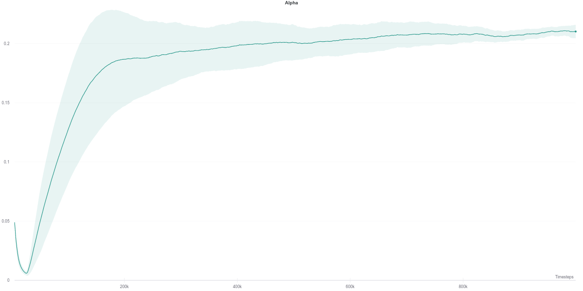
Following the plot above, the auto-tuned entropy version of SAC maintains a value of \(alpha\) around \(0.2\) across its lifetime. Nevertheless, it still manages to achieve a better performance than the agent that uses a fixed value of \(0.2\). However, it is hard to draw any solid conclusion from this observation, with the small number of seeds used to run the experiment.
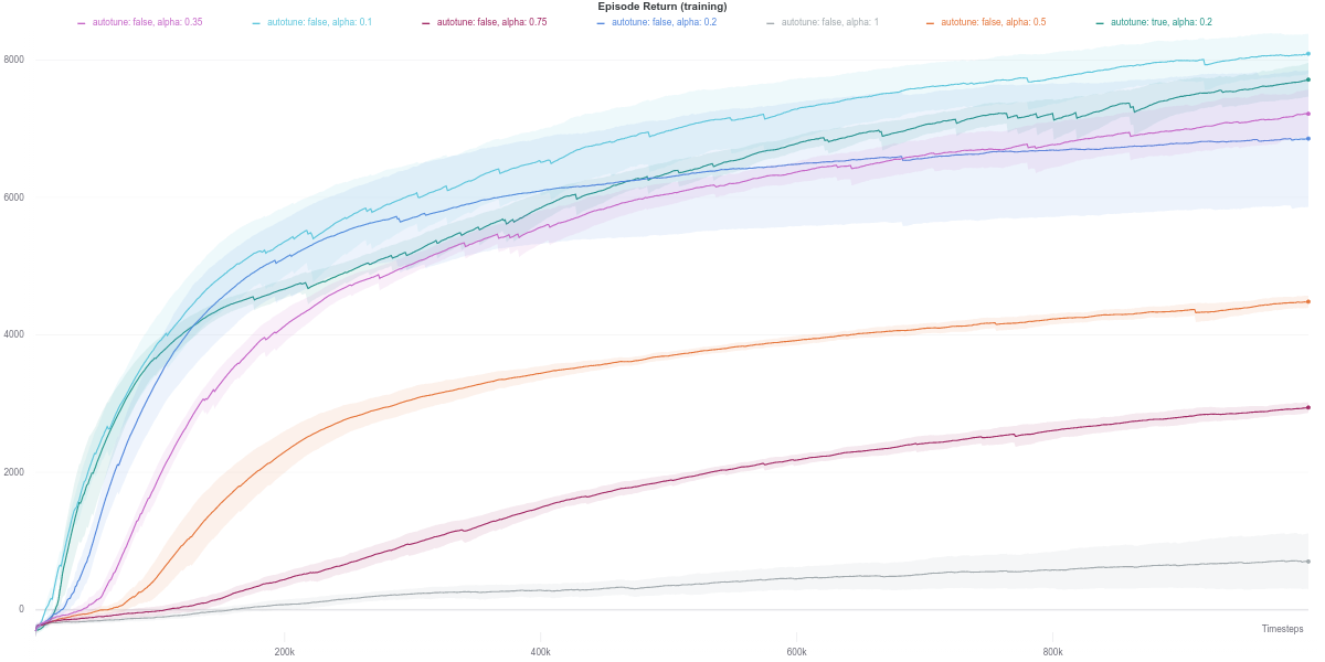
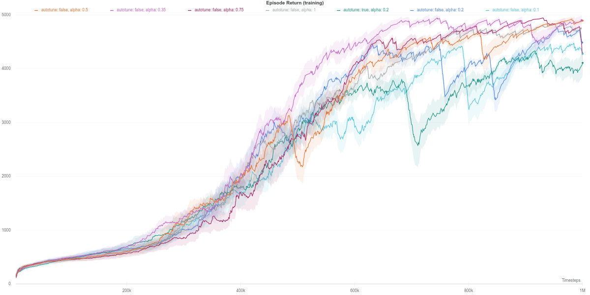
Ant-v2
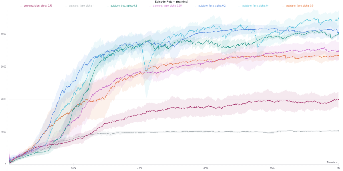
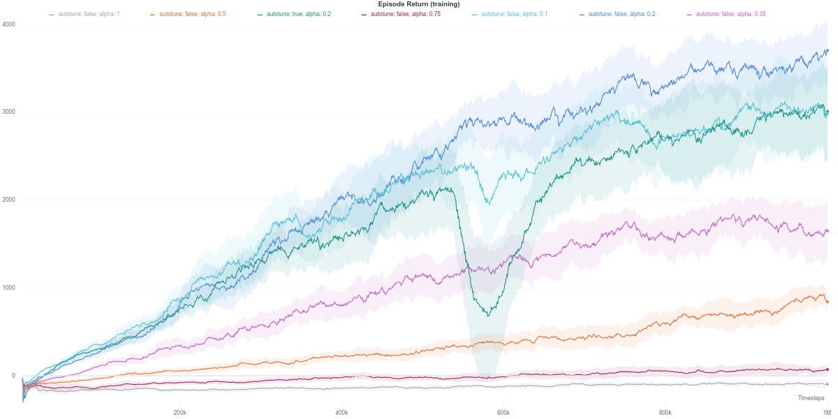
Unlike the relatively simpler environments above, the auto-tuned SAC version displays a slight dip in performance during training, although it does recover by the end of the training. Similar behavior is also observed for the SAC agent with a fixed value $\alpha = 0.1$, but with a smaller magnitude.
The other SAC agents using different values of $\alpha$ do achieve a more stable performance during learning. The best performance is achieved by the SAC with a fixed $\alpha$ value of $0.2$, closely followed by the auto-tuned SAC and SAC with $\alpha = 0.1$, which are seemingly tied together.
However, the higher the value of $\alpha$, the lower the final episodic return of the agent. More specifically, values of $\alpha$ above $0.2$ seem to cripple the agent’s performance. Indeed, the higher it is, the more random the policy of the agent. In a task with a relatively high-dimensional action space such as Ant-v2 (8 degrees of freedom), a policy close to random is less likely to yield a good enough control behavior. It is instead more beneficial to follow the optimization objective of the RL paradigm in such a case.
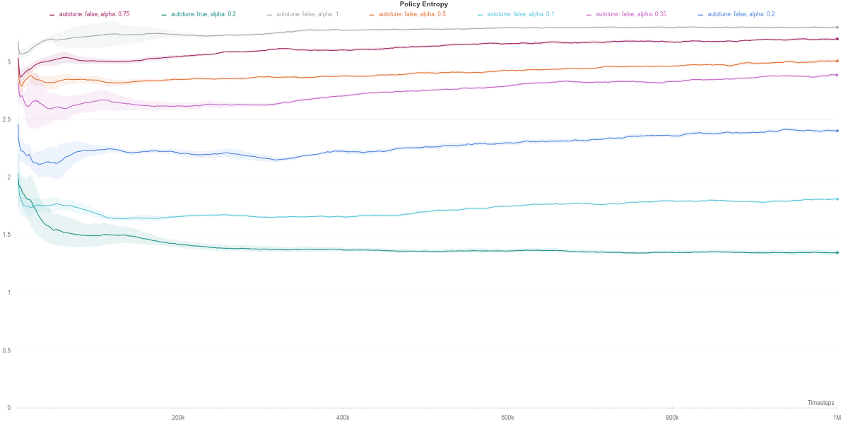
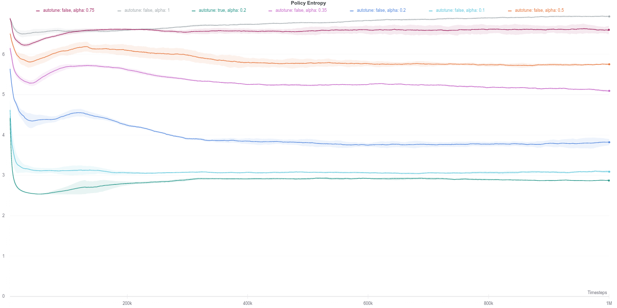
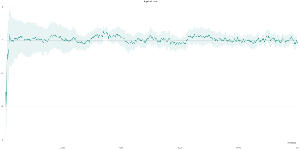
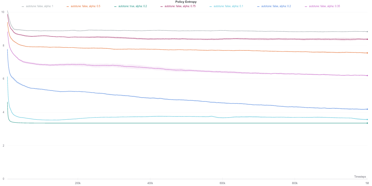
To better understand those dips in performance exhibited by the auto-tuned SAC agent, we start by investigating the various training metrics. First, we observe that the policy entropy is relatively stable for each value of $\alpha$, as well as for the auto-tuned version.
Consequently, the “entropy bonus” that is added the Soft Q-network value in the second equation of the Q-network optimization objective here in the form of \(y = r(s_t, a_t) + \gamma (Q_\theta(s_{t+1},a_{t+1}) - \alpha \text{log} \pi_{\phi}(a_{t+1} \vert s_{t+1}))\) should also be stable.

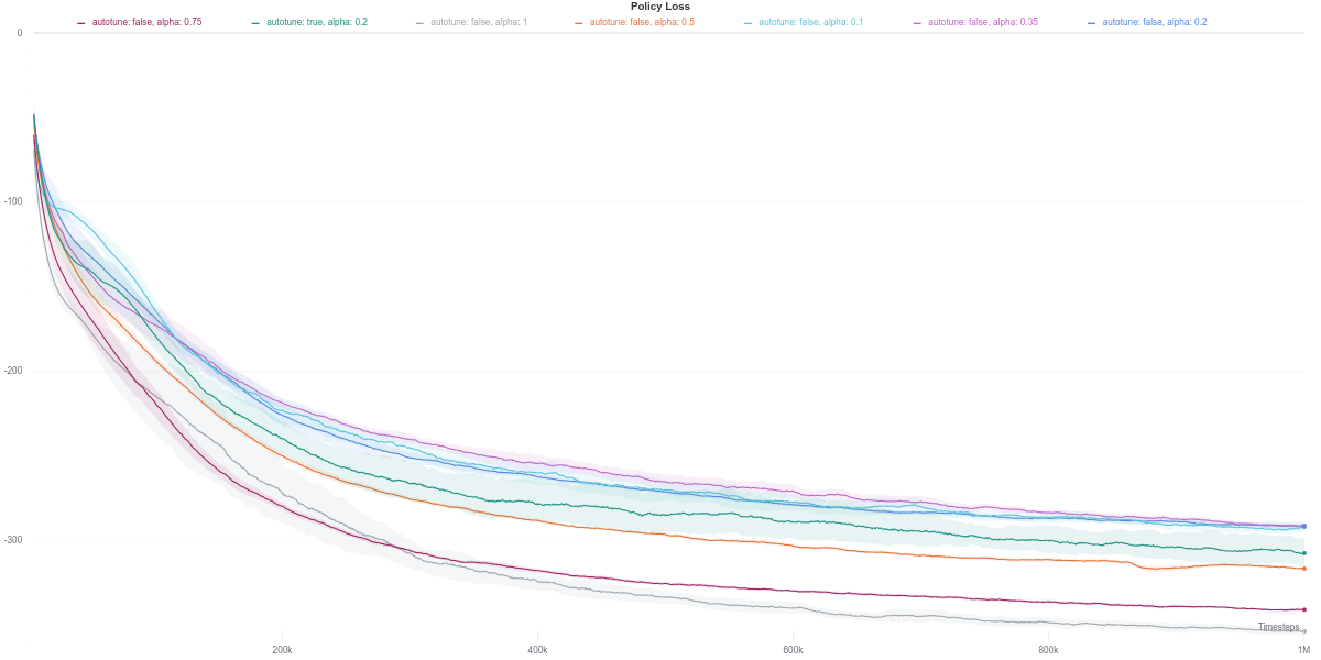
Since the performance of an actor-critic agent is highly dependent on the quality of the critic’s evaluation of the actor’s action, we next investigate the loss of the soft Q-network.
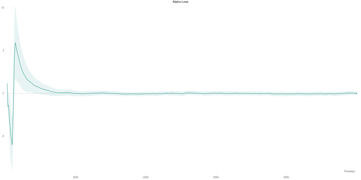
We observe that the Q-network loss for the auto-tuned SAC agent happens to show a large spike right around the time where its performance dips (around the 600K training step mark). Furthermore, this is carried over to the policy loss, where the value of the policy is consequently largely overestimated, which would thus explain the worsening in performance of the agent (figures below). As the quality of the Q-network’s evaluation improves (lower loss), the policy improves correspondingly, leading to the recovery of the agent’s performance.
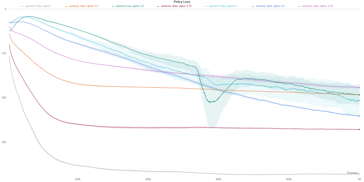
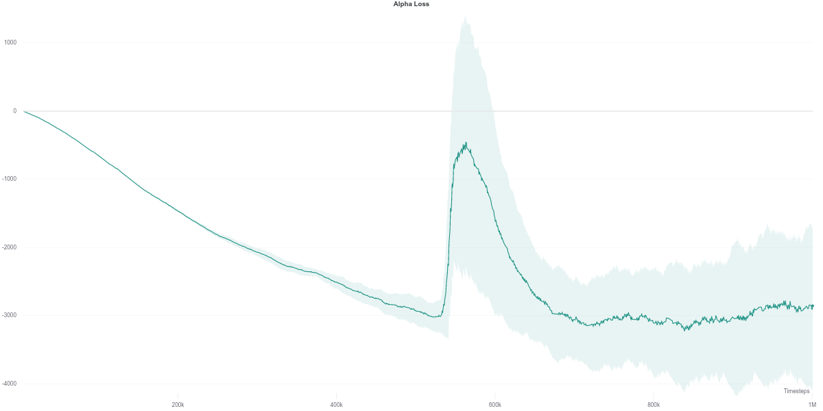
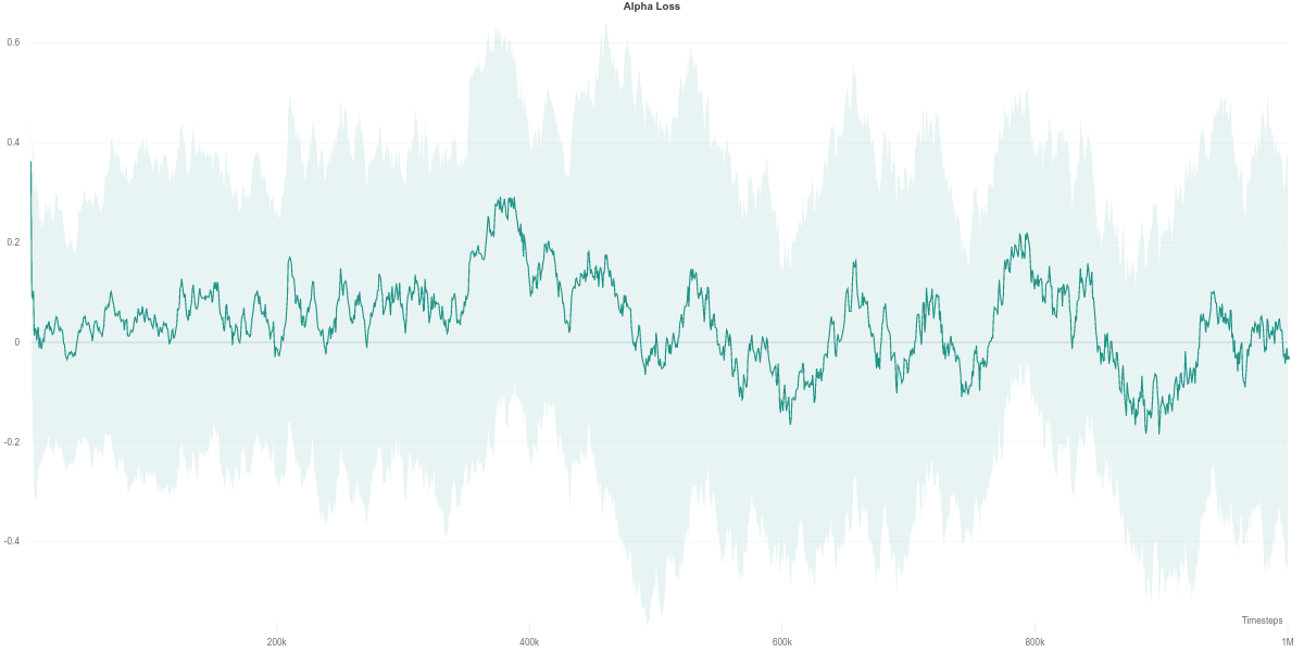
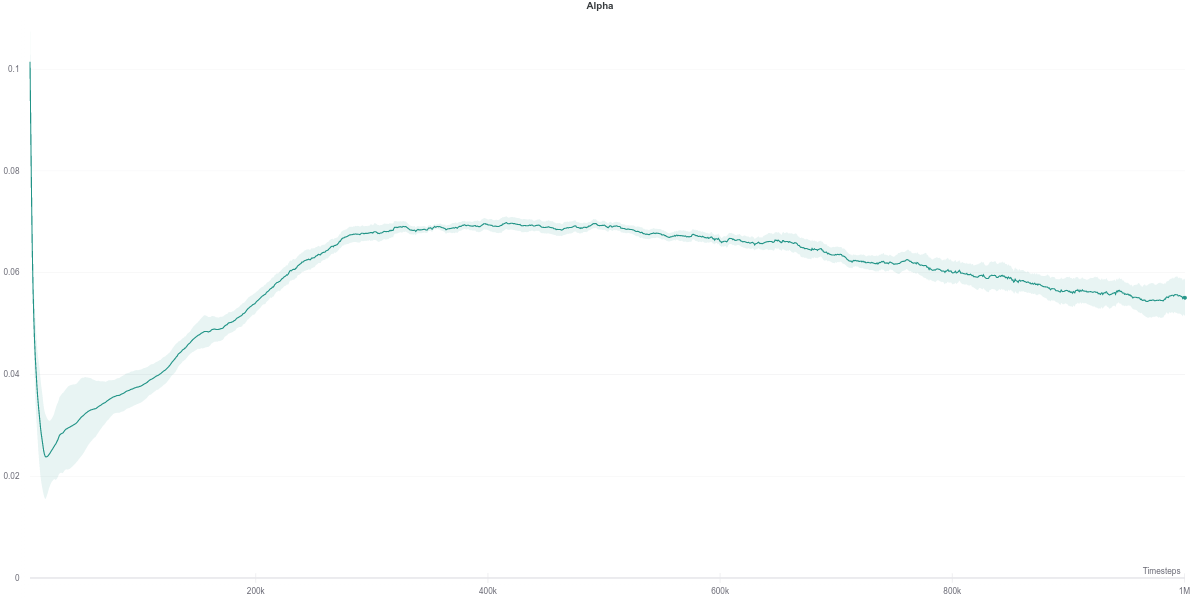
While the $\alpha$ loss is also impacted by the erroneous Q-network evaluation, the value of $\alpha$ does not change around that time frame. Instead, it stays quite low across most of the training time, which makes it equivalent to an entropy-less SAC agent (also similar to $\alpha = 0.1$).
Overall, we see that a small bonus in entropy results in the best performance in this environment. On a final note, it is still hard to say if the automatic tuning of $\alpha$ is really what causes the dip in performance during the training. More empirical results would be desirable before drawing such a conclusion.
Humanoid-v2
The Humanoid environment can be considered as being even more complex than the Ant one. However, the observation of the higher the entropy of the policy, the lower the final agent’s performance does not seem to apply in this case. Namely, the best-performing agents have a relatively high policy entropy, corresponding to values of \(\alpha \in [0.35,1]\). An intuitive interpretation would be that given the complexity of the environment, a high-entropy policy would be better at exploring, thus discovering optimal strategies, than a more conservative policy, for example.
Besides that, while the agents corresponding to lower values do achieve similar performance to the group mentioned above, they seem to be less stable, as per the dips exhibited in their respective learning curves. Moreover, the auto-tuned version of SAC happens to achieve the lowest results out of the lot. In this case, having the lowest entropy does seem to negatively affect the final performance of the agent.
Policy network detailed pseudo-code
This is an over-simplistic, and framework agnostic attempt at describing the various policy network structure encountered while browsing through public repositories. In retrospect, the recap figure should be more helpful to get the overall picture.
1. Original implementation by Tuomas Haarnoja
# Let the observation be defined by x, with a shape of [batch_size, *observation_shape]
# Define a classical MLP feedforward network as the body of the policy.
x = MLP(x)

# Additionally, we a fully connected (FC) layers that outputs the mean and the logstd of the action distribution "jointly"
# Let Da be the dimension of the action space. MeanAndLogStd_FC has an output dimension of 2 * Da
means_and_logstds = MeanAndLogstd_FC(x)
action_means = means_and_logstds[:D] # The first half for the ation means, the latter for the logstds

action_logstds = means_and_logstds[D:] # The second half for the logstd
# Contrary to other implementations which separate the fully connected layers of the means and logstd, the original implementation outputs them jointly.
# There does not seem to be much difference in the results, however.

# Clipping the logstd to the range [-20., 2.]
action_logstds = clip_by_value(action_logstds, -20, 2) # This will block gradients for logstd that are outside of reasonable range.
action_stds = exp(action_logstds) # Apply exponetial to the logstd to recover the standard deviation itself,

# Instantiante the action distribution as a Gaussian parameterized by the previously obtained mean and standard deviations
action_dist = Normal( action_means, action_stds)

# Samples some actions as well as their log probabilities
actions = action_dist.sample()
action_logprobs = action_dist.log_prob( actions)

# The actions are squashed to the [-1, 1] range by defualt with the tanh function.
# It however requires some correction to the action log probabiliities too
actions = tanh(actions)
action_logprobs = logprob_correction( action_logprobs)

# L2 regularization for the policy's weights. https://github.com/haarnoja/sac/blob/8258e33633c7e37833cc39315891e77adfbe14b2/sac/distributions/normal.py#L69

return actions, action_logprobs # The implementation returns deterministic actions (the action_means) that are used for the agent's evaluation.
2. Stable Baselines
This implementation uses a lot of “low-level” techniques to implement the various operations need to compute the action and their log probabilities. But the concept is the same as in the original implementation.
# Let the observation be defined by x, with a shape of [batch_size, *observation_shape]
# Define a classical MLP feedforward network as the body of the policy.
x = MLP(x)

# Additionally, we have two spearate fully connected (FC) layers that output the mean and the logstd of the action distribution, respectively
action_means = ActionMeanFC(x)
action_logstds = ActionLogstdFC(x)

# Clipping the logstd to the range [-20., 2.]
action_logstds = clip_by_value(actions_logstds, -20,2)
action_stds = exp(action_logstds) # Apply exponetial to the logstd to recover the standard deviation itself,

# Instantiate the action distribution as a Gaussian parameterized by the previously obtained mean and standard deviations
action_dist = Normal(action_means, action_stds)

# Samples some actions as well as their log probabilities
actions = action_dist.sample()
action_logprobs = action_dist.log_prob(actions)

# At the time of writing, stable baselines did not seem to implement the L2 regularization for the means and logstd:
# https://github.com/hill-a/stable-baselines/blob/3d115a3f1f5a755dc92b803a1f5499c24158fb21/stable_baselines/sac/policies.py#L219

# Squash the actions to range [-1, 1] and correct the log_probs accordingly
# https://github.com/hill-a/stable-baselines/blob/3d115a3f1f5a755dc92b803a1f5499c24158fb21/stable_baselines/sac/policies.py#L44
deterministic_actions = tanh(action_means)
actions = tanh(actions)
action_logprobs = logprob_correction( action_logprobs)

return deterministic_actions, actions, action_logprobs # Also returns deterministic actions.
Also, note that the Stable Baselines also provide the ability to run SAC on pixel-based environments, namely by upgrading the MLP body of the policy with a CNN feature extractor. That CNN feature extractor is also shared with the Q-network and only updated by the latter during training.
Special notes on the clip_but_pass_gradient() method in SAC
This method is mentioned in the hill-a/stable-baselines and used when applying the corrections to the log probabilities of the actions after the latter have been squashed with the tanh function.
The reason mentioned is to avoid evil machine precision error, which might have been a thing back in the Tensorflow 1.XX days.
This in turn would have led to its removal (comment out, to be more precise), which suggested that either said machine precision error was addressed in subsequent versions of TF, or that it had a negligible impact on the results.
As a memo to myself, its implementation is as follows:
def clip_but_pass_gradient(input_, lower=-1., upper=1.):
    clip_up = tf.cast(input_ > upper, tf.float32)
    clip_low = tf.cast(input_ < lower, tf.float32)
    return input_ + tf.stop_gradient((upper - input_) * clip_up + (lower - input_) * clip_low)
As an aside, this might be useful if used to clip the logstd that contributes to the parameterization of the policy’s action distribution.
Namely, the standard clamping method does not pass any gradient when logstd happens to be outside of the clamping range.
Therefore, there would be no learning signal for the weights of the network that are responsible for the unreasonable logstd values.
The clip_but_pass_gradient could mitigate this issue by providing a small, fixed value as gradient to at least nudge the weights toward better logstd values a little bit faster (?).
3. OpenAI SpinningUp
# Let the observation be defined by x, with a shape of [batch_size, *observation_shape]
# Define a classical MLP feedforward network as the body of the policy.
x = MLP(x)

# Additionally, we have two spearate fully connected (FC) layers that output the mean and the logstd of the action distribution, respectively
action_means = ActionMeanFC(x)
action_logstds = ActionLogstdFC(x)

# Clipping the logstd to the range [-20., 2.]
action_logstds = clamp(action_logstds, -20, 2) # Torch equivalent of clip_by_value.
action_stds = exp(action_logstds) # Apply exponetial to the logstd to recover the standard deviation itself,

# Instantiate the action distribution as a Gaussian parameterized by the previously obtained mean and standard deviations
action_dist = Normal( action_means, action_stds)

# Samples some actions as well as their log probabilities
actions = action_dist.sample()
action_logprobs = action_dist.log_prob( actions)

# Squash the actions and scale them in case the action space is not [-1, 1.]
deterministic_actions = tanh(action_means)
actions = tanh(actions)
action_logprobs = logprob_correction( action_logprobs)

# Scale the actions to match the original action space
actions = action_limit * actions

return actions, action_logprobs # Also return deterministic actions, depending on a flag passed when sampling the actions.
4. Denis Yarats implementation
Probably one of the early Pytorch implementations of the SAC, it follows the original implementation of the author (namely on how it output the joint action means and logstd).
Furthermore, instead of clipping the logstd, it uses the alternative method to cap it, which seems to have been proposed in OpenAI (as per this comment).
Furthermore, it seems to be the only implementation that additionally applies a tanh to the logstd before shifting them in the bounding interval, as well as different values for the bounding interval ([-5,2] instead of the “traditional” [-20,2]).
# Let the observation be defined by x, with a shape of [batch_size, *observation_shape]
# Define a classical MLP feedforward network as the body of the policy.
x = MLP(x)

# Additionally, we a fully connected (FC) layers that outputs the mean and the logstd of the action distribution "jointly"
# Let Da be the dimension of the action space. MeanAndLogStd_FC has an output dimension of 2 * Da
means_and_logstds = MeanAndLogstd_FC(x)
action_means = means_and_logstds[:D] # The first half for the ation means, the latter for the logstds

action_logstds = means_and_logstds[D:] # The second half for the logstd
action_logstds = tanh(action_logstds)

# Let LOG_STD_MIN=-5, LOG_STD_MAX=2
action_logstds = LOG_STD_MIN + 0.5 * (LOG_STD_MAX - LOG_STD_MIN) * (action_logstds + 1)

action_stds = exp(action_logstds)

# Instantiate the action distribution as a Gaussian parameterized by the previously obtained mean and standard deviations
action_dist = Normal( action_means, action_stds)
deterministic_actions = tanh(action_means)
actions = tanh(actions)
action_logprobs = logprob_correction( action_logprobs)
# Note however that this part is done using Pytorch distributions combined with some "advanced" techniques:
# https://github.com/denisyarats/pytorch_sac/blob/815a77e48735416e4a25b44617516f3f89f637f6/agent/actor.py#L41

return actions, action_logprobs, determinsistic_actions
Leave a comment